Text Analysis of the Riksbank Minutes: Insights into the Past, Present and Future

Table of Contents

• Introduction
• Setup
• Data Collection
• Python Integration and Configuration
  • Spacyr Library
  • FinBERT Model
• Data Parsing
• Exploring the Data
  • Sentiment Analysis
  • Word and Bigram Counting
  • TF-IDF Scores
  • Correlation
  • Latent Dirichlet Allocation (LDA)
• Modelling
  • Data Preprocessing
  • Ordered Probit Model
• Conclusion

Introduction

This report presents a text analysis of the Riksbank’s Meetings Minutes, using a vast range of techniques. We explore word counting, correlation analysis, Latent Dirichlet Allocation models, TF-IDF scores and sentiment analysis using Artificial Intelligence. Finally, we estimate a model to assess if sentiment in the minutes can help forecast Monetary Policy movements.

Setup

Note: All required packages are loaded below. Messages and warnings are suppressed for clarity.

# General data wrangling and visualization
library(tidyverse)
library(zoo)
library(ggraph)
library(igraph)
library(ggwordcloud)
library(scales)

# Text mining and topic modeling
library(tm)
library(tidytext)
library(topicmodels)
library(lda)

# Python wrapper for R
library(reticulate)

# NLP (spaCy)
library(spacyr)

# Text co-occurrence and similarity
library(widyr)

# Web scraping and API requests
library(httr2)
library(rvest)

# Wrapper for SCB 
library(pxweb)

# Excel and PDF handling
library(openxlsx)
library(pdftools)

# Set locale to English for date/time functions
invisible(Sys.setlocale("LC_TIME", "C"))

Data Collection

To gather the data, we need to scrappe the Riksbank website. The minutes are available at two different sources:

• Riksbank Website: Minutes from 2017 onwards
• RIksbank Online Archive: Minutes from 1999 to 2016.

Nowadays, the Riksbank holds eight Monetary Policy Meetings a year, but this has changed a lot throughout the years.

The following code provides a function to scrappe the links to the PDFs of the Minutes from both the sources mentioned, alongisde the date they were made available to the public, not the date of the meeting itself. The function follows the same logic as the webscrappes made in my latest publication

fetch_url <- function(page_num, archive = FALSE) {

  # If using the Riksbank's website
  if (archive == FALSE) {
    
     # If page number is 1, use base URL
    if (page_num == 1) {
       url = "https://www.riksbank.se/en-gb/press-and-published/minutes-of-the-executive-boards-monetary-policy-meetings/"
    } else {
    # For page > 1, append page number as a query string
      url = paste0("https://www.riksbank.se/en-gb/press-and-published/minutes-of-the-executive-boards-monetary-policy-meetings/?&page=",page_num,"")
    }
  
    # Scrape all PDF page links from the listing block
    links <- read_html(url) %>% 
      html_elements("div[class='listing-block__body']") %>% 
      html_elements("li") %>%
      html_elements("a") %>%
      html_attr("href") 
    
    text <- read_html(url) %>% 
      html_elements("div[class='listing-block__body']") %>% 
      html_elements("li") %>%
      html_elements("a") %>%
      html_text
    
    # Scrape corresponding dates for each link
    dates <- read_html(url) %>% 
      html_elements("div[class='listing-block__body']") %>% 
      html_elements("li") %>%
      html_elements("a") %>%
      html_elements("span[class='label']") %>% 
      html_text()
    
    # Create data frame and complete the full PDF URL
    df <- bind_cols(date = dates, pdf_links = links, text = text) %>% 
     mutate(pdf_links = (paste0("https://www.riksbank.se/",pdf_links,""))) 
    

  } else if (archive == TRUE) {
   # If using the Riksbank archive
   url = "https://archive.riksbank.se/en/Web-archive/Published/Minutes-of-the-Executive-Boards-monetary-policy-meetings/index.html@all=1.html"
  
    # Scrape links to individual meeting pages
 links <- read_html(url) %>% 
     html_elements("td") %>%
     html_elements("a") %>%
     html_attr("href") 
 
  text <- read_html(url) %>% 
     html_elements("td") %>%
     html_elements("a") %>%
     html_text
  
    # Scrape publication dates
 dates <- read_html(url) %>% 
     html_elements("td") %>%
     html_elements("time") %>% 
     html_text() 
 
    # Combine dates and links into a data frame and fetch the PDF URLs
 df <- bind_cols(date = dates, links = links, text = text) %>% 
    mutate(links = (paste0("https://archive.riksbank.se/en/Web-archive/Published/Minutes-of-the-Executive-Boards-monetary-policy-meetings/",links,""))) %>% 
    mutate(
      # For each meeting page, find the direct PDF link
      pdf_links = map(links, ~ read_html(.x) %>% 
    html_elements("a") %>%
    html_attr("href") %>% 
    .[grep("pdf", .)])
    ) %>% 
    filter(pdf_links != "character(0)") %>%  # Remove meetings without PDF
    unnest(pdf_links) %>%                    # Expand lists into rows
    filter(!grepl("Rapporter", pdf_links)) %>%  # Exclude monetary policy report links (they contamine our sample)
    mutate(pdf_links = gsub("http://archive.riksbank.se/", "", pdf_links)) %>% 
    mutate(pdf_links = (paste0("http://archive.riksbank.se/",pdf_links,""))) %>% 
    select(-links)
   
  }
    # Return final data frame with dates and PDF URLs
  return(df)
}

I then run the function twice, to fetch from each source and bind the data later. After that, I need to make a very ugly correction to dates. The dates we fetch are the dates Meeting Minutes are published, not the day the meeting happens. This generates a conflict with the policy rate, as sometimes minutes are published after actual rates changed and sometimes not. Therefore, we need to adjust by getting the text of each minute link. Their format is not consistent across the whole sample, which leads to all these changes. For three dates, it is necessary to manually input the date

new_links <- map(c(1:6), fetch_url) %>% reduce(bind_rows)
old_links <- fetch_url(page_num="", archive = TRUE)

pattern <- str_c(
  "\\b\\d{1,2}\\s+(?:", paste(month.name, collapse="|"), ")(?:\\s+\\d{4})?\\b",
  "|\\b(?:", paste(month.name, collapse="|"), ")\\s+\\d{1,2}(?:,?\\s*\\d{4})?\\b"
)

links <- bind_rows(new_links, old_links) %>% 
  mutate(date = dmy(date)) %>% 
  arrange(date) %>% 
  unique %>% 
  mutate(date_holder = str_extract(text, regex(pattern, ignore_case=TRUE))) %>% 
  mutate(date_holder = case_when(!grepl("\\b(?:[12][0-9]{3})\\b", date_holder) & !grepl("ecember", date_holder) &
                             !is.na(date_holder) ~ paste(date_holder, year(date)), 
                         !grepl("\\b(?:[12][0-9]{3})\\b", date_holder) & grepl("ecember", date_holder) & 
                           month(date) & !is.na(date_holder) == 12 ~ paste(date_holder, year(date)),
                         !grepl("\\b(?:[12][0-9]{3})\\b", date_holder) & grepl("ecember", date_holder) & 
                           month(date) & !is.na(date_holder) != 12 ~ paste(date_holder, year(date)-1),
                         T ~ date_holder)) %>% 
  mutate(date_holder = case_when(grepl("^[0-9]{1,2} [A-Za-z]+ [0-9]{4}$", date_holder) ~ dmy(date_holder),
                                   grepl("^[A-Za-z]+ [0-9]{1,2} [0-9]{4}$", date_holder) ~ mdy(date_holder),
      T ~ NA)) %>% 
  mutate(date_holder = case_when(date == "2009-02-10" ~ date,
                                 date == "2020-10-01" ~ as_date("2020-09-21"),
                                 date == "2023-02-20" ~ as_date("2023-02-09"),
                                 T ~ date_holder)) %>% 
  mutate(date = date_holder) %>% 
  select(-date_holder, - text)

Then, it is necessary to use the package pdftools to extract the text from each of the Minutes.

minutes <- links %>%
  rowwise %>% 
  mutate(text = list(pdf_data(pdf_links)) %>% 
           bind_rows %>% 
           reframe(text = paste(text, collapse = " ")) %>% 
           pull(text))

Python Integration and Configuration

Spacyr Library

Now that we have all the sentences, it is important to parse the data in an useful and convenient way. For this purpose, I use the spacyr package. It is an R interface to the spaCy natural language procession library in Python, with lots of useful features. For this work especifically, we are interested in the function spacy_parse(), which can parse sentences into structured linguistic data. We are mainly interest in the lemmatization and Part-of-Speech tagging that the function provides.

Installing and activating spacy in an R envinronment is not simples, though. The package is not currently being mantained and I faced issues setting up the package. What worked for me was installing an older version and downgrading the pydantic library to a version earlier than 2.0. This is all done using the reticulate R library. spacy_install() sets up a virtual envinronment of Python named r-spacyr and installs all the necessary features for the model to run. spacy_initialize then initializes the desired model. We are interested in the english one.

Code for installation of spacyr is commented as it only needs to be ran once.

### spacy_install(version = "3.7.4")

# # Caminho para sua virtualenv do spacyr
# venv_path <- "~/.virtualenvs/r-spacyr"
# 
# # 1. Ativa a virtualenv
# reticulate::use_virtualenv(venv_path, required = TRUE)
# 
# # 2. Instala pydantic < 2.0
# reticulate::py_install("pydantic<2.0", envname = venv_path, pip = TRUE)

spacy_initialize(model = "en_core_web_sm")

FinBERT Model

I also use Python to run the AI sentiment analysis model. The model chosen for this task is the FinBERT, a version of Google’s 2018 BERT trained on financial text. This was the undisputed state-of-the-art model for financial sentiment analysis before the introduction of LLMs such as ChatGPT and it is still widely used in literature Taskin; Akal 2024. There is no consensus on whether, right now, if new AI models can perform better than FinBERT in financial sentiment analysis. Zhang; Shen 2024 find that GPT-4o might be as competent as FinBERT, requiring no fine-tuning. Kang; Choi 2025 show that GPT-4o can outperfm FinBERT by 10% only with prompt engineering depending on the sector. Leippold 2023 finds FinBERT is more resilient to adversarial manipulation than GPT3. Nasiopoulos et. al 2025 find that GPT4o and GPT4o-mini can outperform BERT and FinBERT when fine-tuned, but FinBERT shows advantage on handling neutral sentiments.

I opt for FinBERT in this article because it is free, faster and still produces good results. The model hasn’t been updated for a while, so installation might be tricky. To run the model, we need to install the tensorflow, transformers, PyTorch and flax libraries. The following versions worked for me, but the process involved a lot of trial and error, as with the latest versions, crucial DLL and wheels were constantly missing. I’ll leave the installation of the required packages commented as it has to be done only once.

# reticulate::py_install(c(
#   "tensorflow==2.16.1",        
#   "transformers==4.37.2",     
#   "numpy==1.24.4",            
#   "torch",
#   "flax"
# ), pip = TRUE)

After that, it is necessary to configure the FinBERT model. In the first line, I import the BERT model from transformers and in the second line the pipeline function, necessary for running NLP tasks. We then load the model trained on financial data from Hugging Face hub, FinBERT.

from transformers import BertTokenizer, BertForSequenceClassification
from transformers import pipeline

finbert = BertForSequenceClassification.from_pretrained('yiyanghkust/finbert-tone',num_labels=3)
tokenizer = BertTokenizer.from_pretrained('yiyanghkust/finbert-tone')

Data Parsing

Now, I use tidytext, followed by spacyr to parse the data. First, I unnest the full text of the minutes into sentences. After that, we lemmatize all the words and keep only nouns, verbs, adjectives, adverbs and proper names. We then remove dates. Finally, we remove some special characters that bypass the filters and the names of members of the Riksbank Board, as they appear repeatedly in the minutes and do not add relevant information to lemma/word analysis. This will also exclude sentences that contain NONE of these part-of-speeches or ONLY have dates or Board Member names, as they are not relevant for our analysis too.

riksbank_board_members <- c(
  "urban", "bäckström",
  "lars", "heikensten",
  "eva", "srejber",
  "villy", "bergström",
  "kerstin", "hessius",
  "lars", "nyberg",
  "kristina", "persson",
  "irma", "rosenberg",
  "stefan", "ingves",
  "svante", "öberg",
  "barbro", "wickman", "parak",
  "lars", "svensson",
  "karolina", "ekholm",
  "kerstin", "af", "jochnick",
  "per", "jansson",
  "martin", "flodén",
  "cecilia", "skingsley",
  "henry", "ohlsson",
  "erik", "thedéen",
  "anna", "breman",
  "anna", "seim",
  "aino", "bunge"
)

parsed_minutes <- minutes %>%
  unnest_tokens(output = sentences, input = text, token = "sentences") %>% 
  mutate(parsed = list(spacy_parse(sentences) %>%
                         filter(pos %in% c("NOUN", "VERB", "ADJ", "ADV", "PROPN")) %>%
                         filter(!entity %in% c("DATE_I", "DATE_B")) %>% 
                         filter(!token %in% c("%", "§")) %>%
                         filter(!token %in% riksbank_board_members) %>% 
                         select(token, lemma) %>%
                         rename("word" = "token")%>%
                         mutate(across(everything(), function(x) tolower(x)))))  %>%
  unnest(parsed)%>% 
  ungroup 

After parsed, we keep a dataset with only the sentences that bring some sort of information.

data_sentences <- parsed_minutes %>% 
  select(pdf_links, date, sentences) %>%
  unique 

sentences <- data_sentences %>% 
  pull(sentences)

Exploring the Data

Sentiment Analysis

I now run the FinBERT model in python. This takes a while to run, as there are a lot of sentences

nlp = pipeline("sentiment-analysis", model=finbert, tokenizer=tokenizer)

results = nlp(r.sentences)

When the results are available, I organize the results into an R dataframe. Each sentence has a label defining whether it is positive, negative or neutral, following a score on the intensity of each category. After that, it is possible to create an index and showcase it in a graph.

data_sentiment_bert <- 
  py$results %>%
  bind_rows %>%
  bind_cols(data_sentences, .)

data_sentiment_bert  %>% head(5)

## # A tibble: 5 × 5
##   pdf_links                                     date       sentences label score
##   <chr>                                         <date>     <chr>     <chr> <dbl>
## 1 http://archive.riksbank.se/../../../../../..… 1999-04-08 8 separa… Neut… 1.00 
## 2 http://archive.riksbank.se/../../../../../..… 1999-04-08 the riks… Neut… 0.999
## 3 http://archive.riksbank.se/../../../../../..… 1999-04-08 he there… Neut… 1.00 
## 4 http://archive.riksbank.se/../../../../../..… 1999-04-08 the exec… Neut… 1.00 
## 5 http://archive.riksbank.se/../../../../../..… 1999-04-08 this min… Neut… 1.00

db_graph <- data_sentiment_bert %>%
  ungroup %>%
  mutate(date = as_date(as.yearmon(date))) %>%
  arrange(date) %>%
  mutate(label = case_when(label == "Negative" ~ -1,
                           label == "Neutral" ~ 0,
                           label == "Positive" ~ 1)) %>% 
  reframe(sentiment = mean(score*label),
          .by = date) %>%
  mutate(sentiment = scale(sentiment)[,1]) %>%
  mutate(sentiment = rollmeanr(sentiment,3,NA)) %>%
  na.omit

g1 <-   ggplot(db_graph,
               aes(date, sentiment, fill = sentiment>0)) +
  geom_col(show.legend = FALSE) +
  scale_fill_manual(values=c("#006AA7","#FECC02"))+
  theme_minimal() + xlab("") + ylab("") +
  scale_x_date(date_labels = "%Y",
               breaks = seq(from = as.Date(paste(year(min(db_graph$date)),
                                                 month(min(db_graph$date)),
                                                 "01",
                                                 sep="-")),
                            to = max(db_graph$date), length.out=10),
               expand = expansion(mult = c(0.01,0.01))) +
  scale_y_continuous(n.breaks = 8) +
  labs(title="Sentiment in Riksbank Minutes",
       subtitle = "FinanceBERT AI Sentiment Scores, Z-Score, 3MMA",
       caption = "Source: Riksbank and Own Calculations") +
  theme(panel.grid.major.x = element_blank(),
        panel.grid.minor.x = element_blank(),
        panel.grid.major.y = element_line(colour="lightgray", size=0.1),
        panel.grid.minor.y = element_line(colour="lightgray", size=0.1),
        legend.position = "none",
        axis.text.x = element_text(angle = 90, vjust = 0.5, hjust=1),
        plot.title=element_text(face="bold"),
        legend.title=element_blank()) +
  guides(col = guide_legend(direction = "horizontal"),
         shape = guide_legend(direction = "horizontal")) +
  theme(legend.position=c(1, 1.015),
        legend.justification="right",
        plot.title = element_text(vjust = 1.5),
        plot.subtitle = element_text(vjust = 3.75),
        strip.text.x = element_blank())

g1

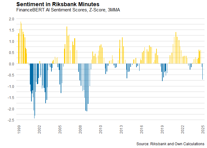
The FinanceBERT results map closely onto Sweden’s real-world cycles.

In the late 1990s, optimism soared as the country emerged from an early 90s fiscal and banking crisis: balanced budgets, low rates and an export led by R&D boom drove unemployment down and confidence up.

The dot-com bust then plunged sentiment into negative territory, as exports slumped and worries about the Eurozone rose. This is the period when Germany, Sweden’s largest trading partner, was nicknamed “Sickman of Europe”

From 2005 to 2007, buoyant global demand, low interest rates and the commodity boom reignited optimism, only for the Global Financial Crisis to send it into a deep trough again.

Modest recovery in the early 2010s gave way to renewed caution, with some downticks in 2012 amid the Euro-debt crisis

2014–18 brought solid growth, falling unemployment and inflation at or below target, restoring a broadly positive tone.

2019’s trade-war concerns and the COVID-19 pandemic in 2020 drove sentiment back to negative, before a strong 2021 rebound, fueled by vaccinations, the economy reopening and spending of excess savings.

Finally, 2022’s inflation spike and 2023’s sluggish growth tempered sentiment once more. In 2024 inflation returned to target and the Riksbank was able to cut rates, renewing optimism in the minutes, even though unemployment remained very high and growth under pre-COVID levels. Finally, 2025’s U.S. tariff threats quickly shifted tone to negative territory, reaching the worst since the pandemic.

loughran_sentiment <- tidytext::get_sentiments("loughran") %>% 
  rename("lemma" = "word") %>% 
  filter(sentiment %in% c("negative", "positive"))


data_sentiment_loug <- parsed_minutes %>% 
  select(date, lemma) %>% 
  inner_join(loughran_sentiment) %>% 
  mutate(date = as_date(as.yearmon(date)))


db_graph <- data_sentiment_loug %>% 
  arrange(date) %>% 
  reframe(count = n(),
          .by = c(date, sentiment)) %>% 
  pivot_wider(names_from = sentiment, values_from = count) %>% 
  reframe(date, polarity = (positive-negative)/(positive+negative)) %>% 
  mutate(polarity = scale(polarity)[,1]) %>% 
  mutate(polarity = rollmeanr(polarity,3,NA)) %>% 
  na.omit


g2 <-   ggplot(db_graph,
               aes(date, polarity, fill = polarity>0)) +
  geom_col(show.legend = FALSE) +
  scale_fill_manual(values=c("#006AA7","#FECC02"))+
  theme_minimal() + xlab("") + ylab("") +
  scale_x_date(date_labels = "%Y",
               breaks = seq(from = as.Date(paste(year(min(db_graph$date)),
                                                 month(min(db_graph$date)),
                                                 "01",
                                                 sep="-")), 
                            to = max(db_graph$date), length.out=10),
               expand = expansion(mult = c(0.01,0.01))) +
  scale_y_continuous(n.breaks = 8) +
  labs(title="Sentiment in Riksbank Minutes",
       subtitle = 'Customized Loughran Lexicon Polarity,3MMA, Z-Score\nPolarity= (positive-negative)/(positive+negative)',
       caption = "Source: Riksbank and Own Calculations") +
  theme(panel.grid.major.x = element_blank(),
        panel.grid.minor.x = element_blank(),
        panel.grid.major.y = element_line(colour="lightgray", size=0.1),
        panel.grid.minor.y = element_line(colour="lightgray", size=0.1),
        legend.position = "none",
        axis.text.x = element_text(angle = 90, vjust = 0.5, hjust=1),
        plot.title=element_text(face="bold"),
        legend.title=element_blank()) +
  guides(col = guide_legend(direction = "horizontal"),
         shape = guide_legend(direction = "horizontal")) +
  theme(legend.position=c(1, 1.015),
        legend.justification="right",
        plot.title = element_text(vjust = 1.5),
        plot.subtitle = element_text(vjust = 3.75),
        strip.text.x = element_blank()) 

g2

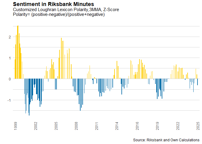
As a benchmark, it is interesting to compare to a simpler word counting model. We use the Loughran-McDonald dictionary for this purpose. With the tidytext package, it is possible to download it simply. We do not need to get the whole sentences as context does not matter for this index

Word and Bigram Counting

Let’s take a look at the frequency of some keywords throughout history

data_count <- parsed_minutes %>% 
  filter(lemma %in% c("wage", "demand", "inflation", "pressure", "unemployment", "activity", "uncertainty", "risk")) %>% 
  mutate(date = as_date(as.yearmon(date))) %>% 
  reframe(count = n(),
          .by = c(date, lemma)) %>% 
  arrange(date)

db_graph <- data_count

g3 <- ggplot(data = db_graph) +
  geom_col(aes(x = date, y = count), fill = "#006AA7") +
  facet_wrap(~lemma, scales = "free", nrow = 2) +
  theme_minimal() + xlab("") + ylab("") +
  scale_y_continuous(breaks = pretty_breaks(n=5)) +
  scale_x_date(labels = date_format("%b %y"), 
               breaks = seq.Date(from=min(db_graph$date),
                                 to=max(db_graph$date),
                                 length.out=13),
               expand = expansion(mult = c(0.01,0.05))) +
  labs(title="Selected Words Frequency",
       subtitle="Units/Numbers",
       caption = "Source: Riksbank and Own Calculations") +
  theme(panel.grid.major.x = element_blank(),
        panel.grid.minor.x = element_blank(),
        panel.grid.major.y = element_line(colour="lightgray", size=0.1),
        panel.grid.minor.y = element_line(colour="lightgray", size=0.1),
        axis.text.x = element_text(angle = 90, vjust = 0.5, hjust=1),
        plot.title=element_text(face="bold"),
        legend.title=element_blank(),
        legend.key.size = unit(0.8, "cm")) +
  theme(legend.box = "horizontal")+ 
  guides(col = guide_legend(direction = "horizontal"),
         fill = guide_legend(direction = "horizontal"),
         shape = guide_legend(direction = "horizontal")) +
  theme(legend.position=c(1, 1.015),
        legend.justification="right",
        plot.title = element_text(vjust = 1.5),
        plot.subtitle = element_text(vjust = 3.75))

g3

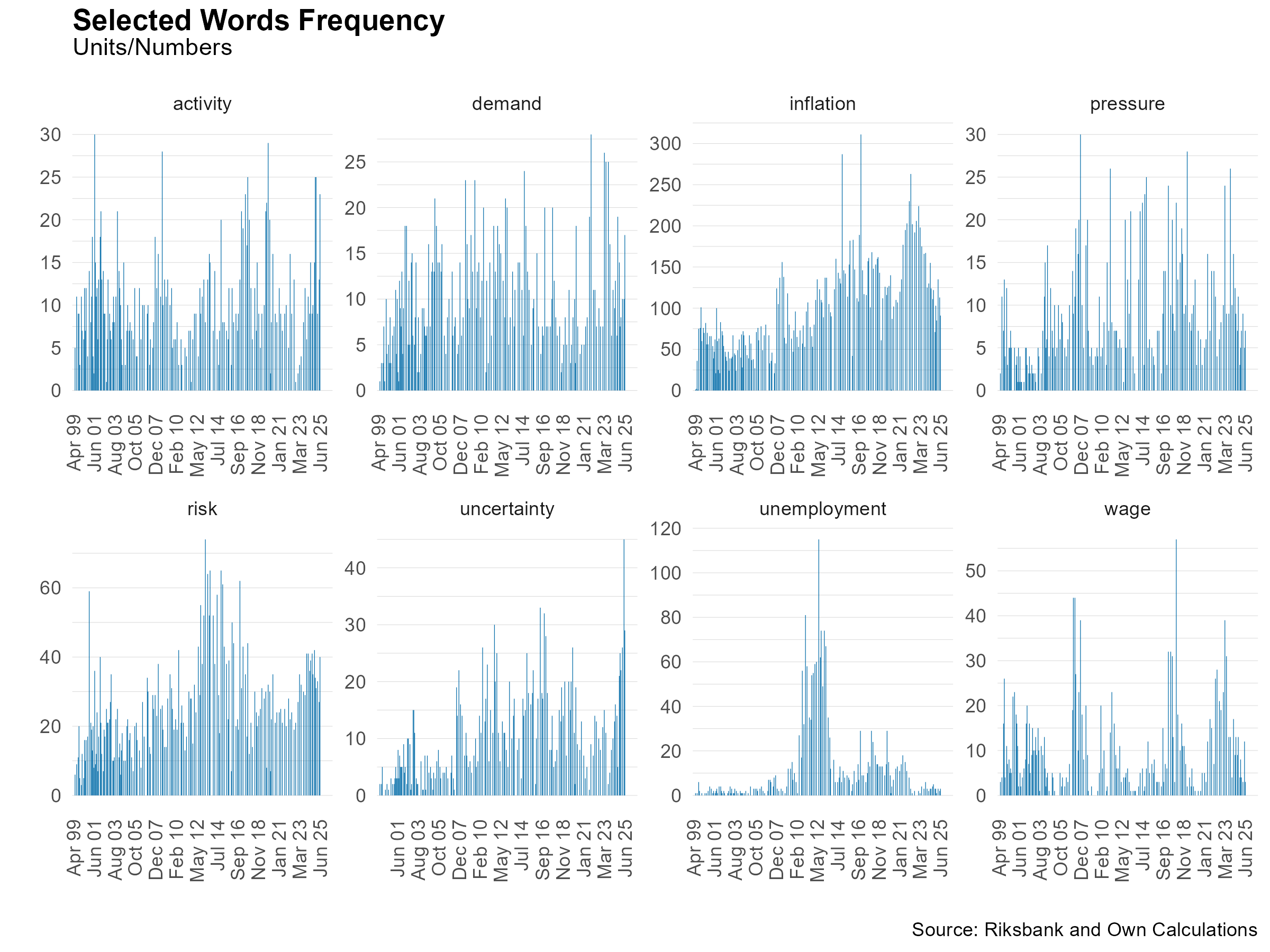
Word counting provides interesting insights on where the Riksbank was focusing at each period in history. Inflation is brought up more frequently during 2022 and 2023, period where it reached over 10%. Trump’s tariffs brought “uncertainty” count to the highest in history. Risk and unemployment spiked during the Euro Debt crisis. Demand and pressure were mentioned a lot during the economy reopening following the pandemic. Activity seems to hit higher levels during economic crisis.

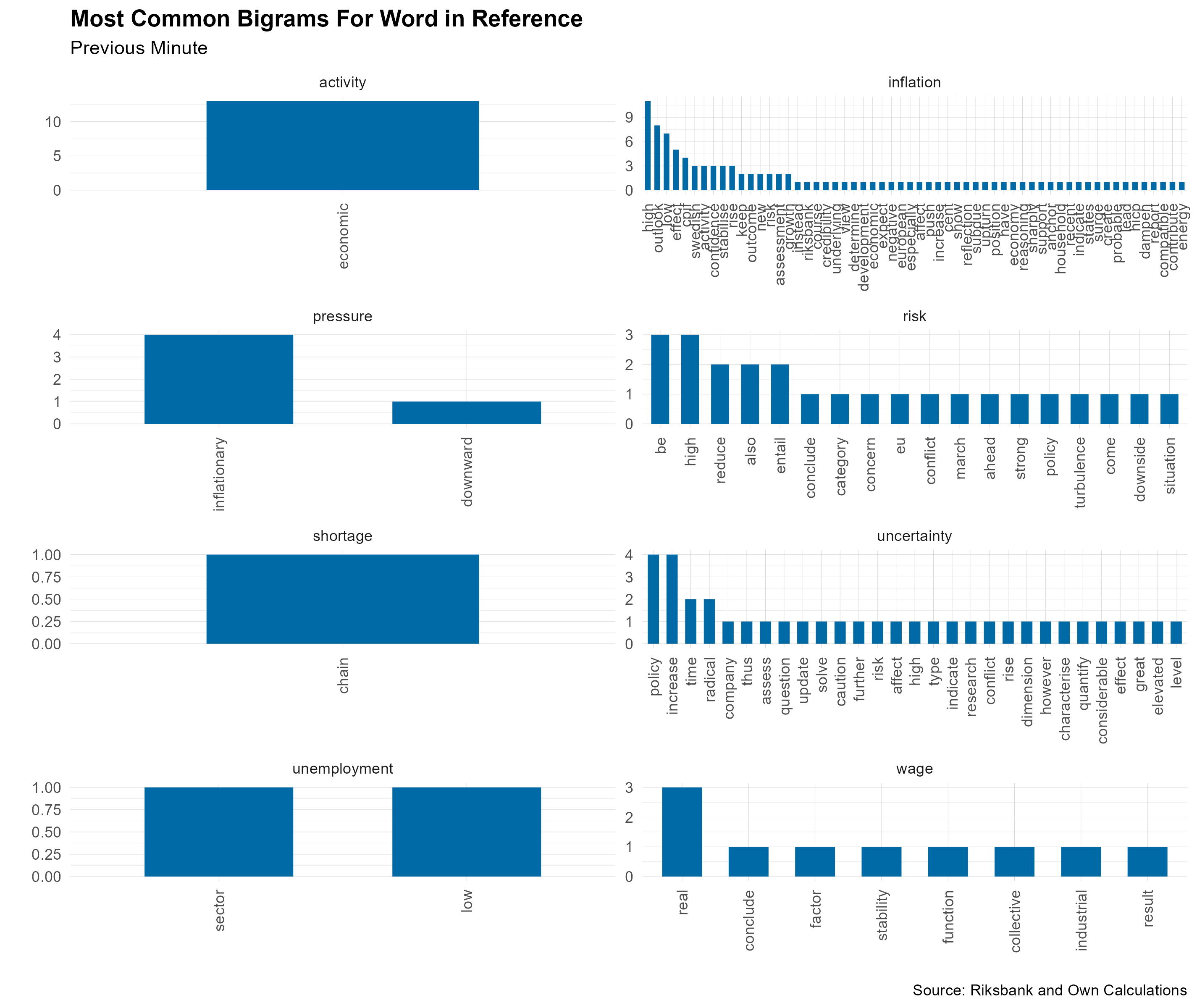
But, of course, words alone don’t tell a full story. It is important to consider context. Hence, the next graphs show which was the most common bigram for the selected words in the two last minutes.

two_last_dates <- distinct(parsed_minutes, date) %>% tail(2) %>% pull(date)

db_graph <- parsed_minutes %>% 
  filter(date %in% two_last_dates) %>% 
  reframe(sentences = paste(lemma, collapse = " "),
          .by = c(date, sentences)) %>% 
  unnest_tokens(output = bigram, input = sentences, token = "ngrams", n =2) %>% 
  separate(bigram, c("word1", "word2"), sep = " ") %>% 
  filter(word2 %in% c("wage", "shortage", "inflation", "pressure", "unemployment", "activity", "uncertainty", "risk")) %>% 
  arrange(date) %>% 
  reframe(count = n(), 
          .by = c(word1, word2, date)) %>% 
  arrange(count) %>% 
  mutate(holder = paste(word1, word2, date, sep = "_")) %>% 
  mutate(holder = factor(holder, levels = rev(holder))) %>% 
  arrange(date)

g4_1 <- ggplot(db_graph %>% filter(date == first(date)), aes(x = holder)) +
  geom_col(aes(y=count), position = "dodge", width=0.6, fill = "#006AA7") +
  facet_wrap(~word2, scales = "free", nrow=4) +
  scale_x_discrete(labels = function(x) gsub("_.+$", "", x))  +
  theme_minimal() + xlab("") +ylab("") +
  labs(title="Most Common Bigrams For Word in Reference",
       subtitle="Previous Minute",
       caption="Source: Riksbank and Own Calculations") +
  theme(panel.grid = element_line(colour="lightgray", size=0.1),
        axis.text.x = element_text(vjust = 0.5, hjust=1,
                                   angle=90),
        plot.title=element_text(face="bold"),
        legend.title=element_blank(),
        legend.key.size = unit(0.5, "cm"),
        legend.position="none")

g4_2 <- ggplot(db_graph %>% filter(date == last(date)), aes(x = holder)) +
  geom_col(aes(y=count), position = "dodge", width=0.6, fill = "#006AA7") +
  facet_wrap(~word2, scales = "free", nrow=4) +
  scale_x_discrete(labels = function(x) gsub("_.+$", "", x))  +
  theme_minimal() + xlab("") +ylab("") +
  labs(title="Most Common Bigrams For Word in Reference",
       subtitle="Latest Minute",
       caption="Source: Riksbank and Own Calculations") +
  theme(panel.grid = element_line(colour="lightgray", size=0.1),
        axis.text.x = element_text(vjust = 0.5, hjust=1,
                                   angle=90),
        plot.title=element_text(face="bold"),
        legend.title=element_blank(),
        legend.key.size = unit(0.5, "cm"),
        legend.position="none")

g4_1

g4_2

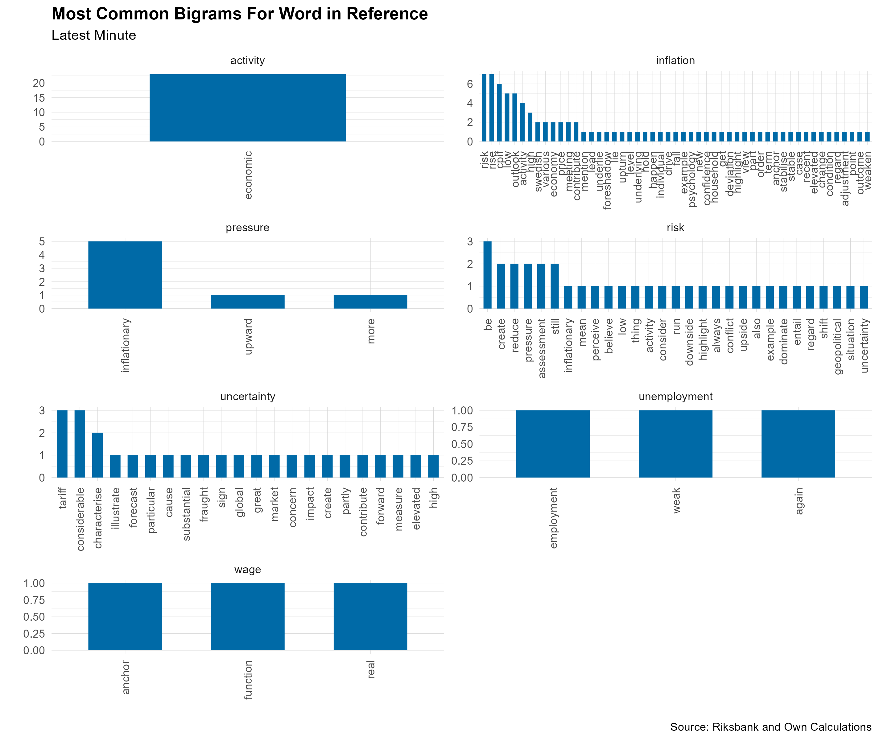
These graphs produce a more marginal and nuanced analysis of the Riksbank focus shift. “High” inflation was substituted by “risk” and “rise”. “Tariff” was not mentioned right before “uncertainty” in the previous minute, with “policy” being the top bigram, but has three mentions on the latest.

Correlation

Adding to the word counting methods, we can calculate pairwise correlation between lemmas. The “feature” column that unites them is the sentences one. Therefore, we are consider lemmas are linked when they are mentioned in the same sentence.

data_net <- parsed_minutes %>% 
  mutate(date = as_date(as.yearmon(date))) %>% 
  arrange(date) %>% 
  filter(date == last(date)) %>% 
  group_by(lemma) %>%
  filter(n() >= 10) %>%
  pairwise_cor(lemma, sentences, sort = TRUE)

g5 <- 
  data_net %>%
  filter(correlation > .25) %>%
  graph_from_data_frame() %>%
  ggraph(layout = "fr") +
  geom_edge_link(aes(edge_alpha = correlation), edge_colour = "#006AA7",show.legend=FALSE) +
  geom_node_point(color ="#006AA7", size = 5) +
  geom_node_text(aes(label = name), repel = TRUE) +
  theme_void() +
  theme(plot.margin = unit(c(rep(.5,4)), "cm"))+
  labs(title="  Pairs of words in Riksbank Minutes that show at\n  least a 0.25 pairwise correlation", caption="  Source: Riksbank and Own Calculations    \n",
       subtitle = "  Latest Minute")

g5

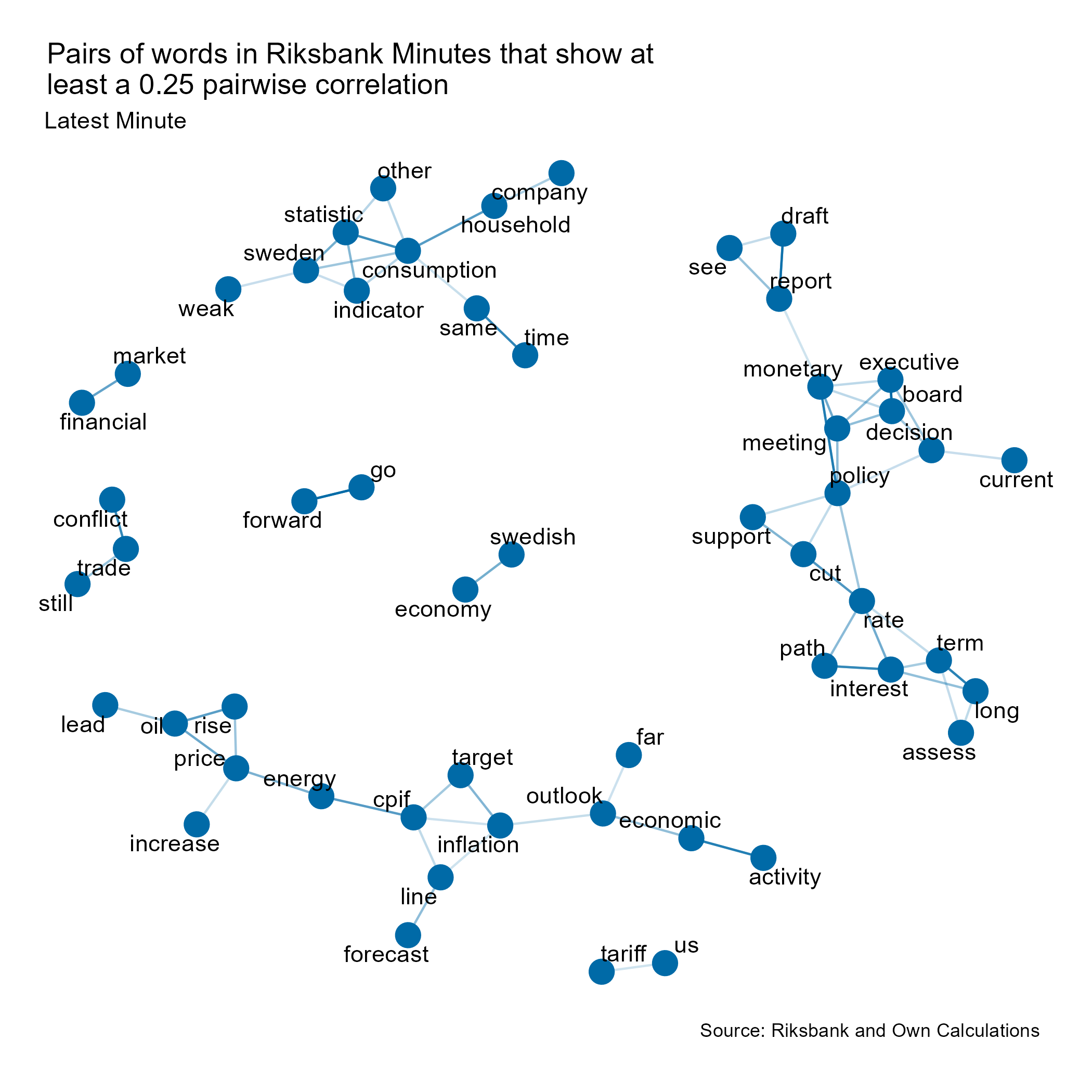
The graph cloud provides a nice visualization on the main topics of the latest Riksbank minute. There are three main clouds connecting a lot of words. In one of them, it is indicated that consumption in Sweden has been weak. Other highlights that rise in oil prices increased energy prices, but CPIF appears to be in line with forecasts. Finally, the Board decided to cut interest rates during the monetary policy meetings. This indicates that downside risks to activity outweighed the risks of higher inflation in the Board’s view. Two smaller clouds, connecting “tariff” to “us” and “conflict” to “trade” to “still” also show that the trade war is on the focus of the Bank’s attention.

TF-IDF Scores

I now proceed to calculate Term Frequency-Inverse Document Frequency scores. This is an important measure in text analysis to assess if a certain word is being relatively more mentioned in a document than in a bigger sample. It complements simple word counting methods and allows a deeper investigation of the Riksbank focuses through time.

To do so, we consider each sentence a document and aggregate it in a corpus. Then, we compute the Document Term Matrix, where each row corresponds to a document, each column a word and each cell the amount of times that the word appeared in the respective document. Remember document here are sentences.

Note: The sentences here are filtered to include only the words left after parsing with spacyr and filtering.

data_lda <- parsed_minutes %>%
  reframe(text = paste(word, collapse = " "), 
          .by = c(date, sentences)) %>% 
  mutate(doc_id = as.character(row_number())) %>%
  relocate(doc_id, text) %>%
  ungroup %>%
  as.data.frame()

data_corpus <- Corpus(DataframeSource(data_lda))

DTM <- DocumentTermMatrix(data_corpus)

empty_rows <- which(slam::row_sums(DTM) == 0)

It is necessary to compute the Document Term Matrix twice, as we need to remove residual sentences with no words, such as “d.” and “b.”, and it is hard to know ex-ante which sentences are these. To do so, we get the row number of every row that all cells correspond to 0. Then, we recalculate removing them before creating the corpus.

data_lda <- parsed_minutes %>%
  reframe(text = paste(word, collapse = " "), 
          .by = c(date, sentences)) %>% 
  mutate(doc_id = as.character(row_number())) %>%
  relocate(doc_id, text) %>%
  ungroup %>%
  as.data.frame() %>% 
  filter(!row_number() %in% empty_rows)

data_corpus <- Corpus(DataframeSource(data_lda))

DTM <- DocumentTermMatrix(data_corpus)

data_lda_lemma <- parsed_minutes %>%
  reframe(text = paste(lemma, collapse = " "), 
          .by = c(date, sentences)) %>% 
  mutate(doc_id = as.character(row_number())) %>%
  relocate(doc_id, text) %>%
  ungroup %>%
  as.data.frame() %>% 
  filter(!row_number() %in% empty_rows)

data_corpus_lemma <- Corpus(DataframeSource(data_lda_lemma))

DTM_lemma <- DocumentTermMatrix(data_corpus_lemma)

I create two Document Term Matrix: the first with words and the second with lemmas.

Note: We calculate the TF-IDF on lemmatized words.

data_tf_idf <- tidy(DTM_lemma) %>% 
  full_join(data_lda %>% rename("document" = "doc_id") %>% select(document,date))

tf_idf_year <- data_tf_idf %>% 
  mutate(year = year(as_date(as.yearmon(date)))) %>% 
  reframe(count = sum(count),
          .by = c(year,term)) %>% 
  bind_tf_idf(term, year, count) %>% 
  arrange(year) %>% 
  reframe(tf_idf = mean(tf_idf),
          .by = c(year,term))

db_graph <- tf_idf_year %>% 
  group_by(year) %>% 
  arrange(desc(tf_idf)) %>% 
  slice_head(n=10) %>% 
  ungroup %>% 
  mutate(holder = paste(term, year, sep = "_")) %>% 
  mutate(holder = factor(holder, levels = rev(holder))) 

g6_1 <- ggplot(db_graph, aes(x = tf_idf)) +
  geom_bar(aes(y=holder),stat="identity",width=0.6, fill = "#006AA7") +
  facet_wrap(~year, scales = "free", ncol = 5) +
  scale_y_discrete(labels = function(x) gsub("_.+$", "", x))  +
  scale_x_continuous(breaks = c(1:max(db_graph$tf_idf))) +
  theme_minimal() + xlab("") +ylab("") +
  labs(title="Highest TF-IDF Words by Year",
       subtitle="TF-IDF is measured with aggregation at year level and only with lemmas",
       caption="Each facet has is own scale
Source: Riksbank and Own Calculations") +
  theme(panel.grid = element_line(colour="lightgray", size=0.1),
        axis.text.x = element_text(vjust = 0.5, hjust=1,
                                   angle=90),
        plot.title=element_text(face="bold"),
        legend.title=element_blank(),
        legend.key.size = unit(0.5, "cm"),
        legend.position="none")

g6_1

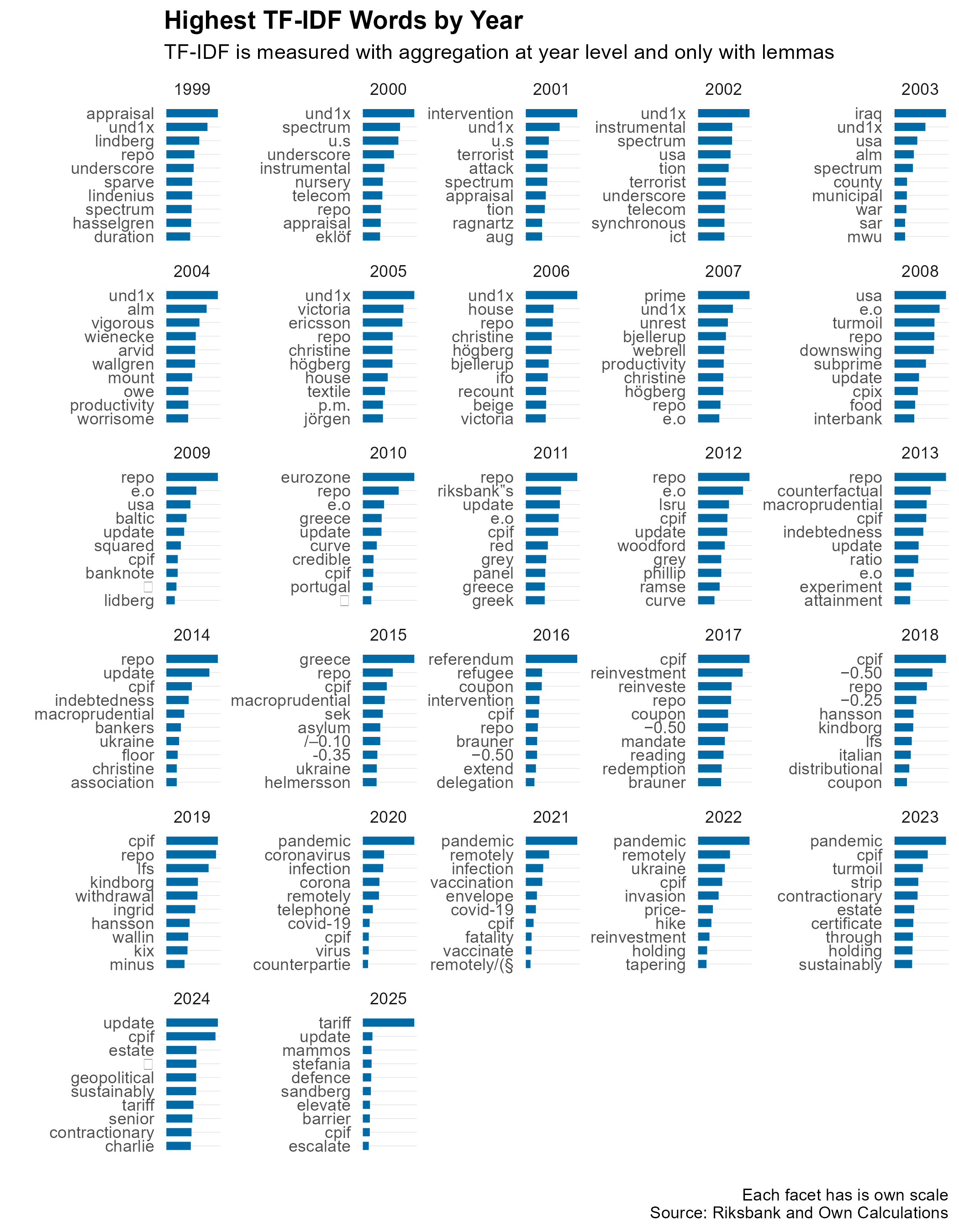
The graph above shows TF-IDF scores considering each year as an unique document. It is useful to tell a broader story and see more long term tendencies. For some periods, scores corroborate with a larger macro picture.

• 2001
  • 9/11 attacks
  • “u.s”, “terrorist”, “attack”
• 2003
  • Iraq war
  • “Iraq”, “USA”, “war”
• 2004–07
  • Growth confidence and telecom exposure
  • “vigorous”, “productive”, “telecom”, “textile”
• 2008–09
  • GFC stress
  • “turmoil”, “interbank”, “depression”, “subprime”, “usa”, “baltic”, “banknote”
• 2010–13
  • Euro‑area struggle and liquidity focus
  • “Eurozone”, “Greek”, “Portugal”, “counterparty”, “repo”
• 2014–16
  • Toolkit evolution: inflation‑measure switch and credit control, Crimea war, Syrian refugee crisis, Greece elections and negotiations, Brexit
  • “macroprudential”, “CPIF”, “bankers”, “intervention”, “ukraine”, “ayslum”, “refugee”, “greece”, “referendum”
• 2020–21
  • Covid-19 crisis
  • “pandemic”, “vaccine”, “refinancing”, “coronavirus”, “covid-19”, “remotely”, “infection”, “wave”, “fatality”
• 2022–23
  • Inflation spike and war
  • “inflation”, “Ukraine”, “invasion”, “price”, “turnoil”, “hike”
• 2024–25
  • Geopolitical uncertainty and US elections
  • “geopolitical”, “tariff”, “election”, “defence”, “elevate”

It is also interesting to note the change of focus from the und1x measure (later renamed CPIX) to the CPIF (which became the official target in mid-2017).

tf_idf_month <- data_tf_idf %>% 
  mutate(date = as_date(as.yearmon(date))) %>% 
  filter(date >= max(date) - months(24)) %>% 
  reframe(count = sum(count),
          .by = c(date,term)) %>% 
  bind_tf_idf(term, date, count) %>% 
  arrange(date) %>% 
  reframe(tf_idf = mean(tf_idf),
          .by = c(date,term))

db_graph <- tf_idf_month %>% 
  group_by(date) %>% 
  arrange(desc(tf_idf)) %>% 
  slice_head(n=10) %>% 
  ungroup %>% 
  mutate(date = as.yearmon(date)) %>% 
  mutate(holder = paste(term, date, sep = "_")) %>% 
  mutate(holder = factor(holder, levels = rev(holder)))

g6_2 <- ggplot(db_graph, aes(x = tf_idf)) +
  geom_bar(aes(y=holder),stat="identity",width=0.6, fill = "#006AA7") +
  facet_wrap(~date, scales = "free", ncol = 5) +
  scale_y_discrete(labels = function(x) gsub("_.+$", "", x))  +
  scale_x_continuous(breaks = c(1:max(db_graph$tf_idf))) +
  theme_minimal() + xlab("") +ylab("") +
  labs(title="Highest TF-IDF Words by Month",
       subtitle="TF-IDF is measured with aggregation at month level and only with lemmas",
       caption="Each facet has is own scale
Source: Riksbank and Own Calculations") +
  theme(panel.grid = element_line(colour="lightgray", size=0.1),
        axis.text.x = element_text(vjust = 0.5, hjust=1,
                                   angle=90),
        plot.title=element_text(face="bold"),
        legend.title=element_blank(),
        legend.key.size = unit(0.5, "cm"),
        legend.position="none")

g6_2

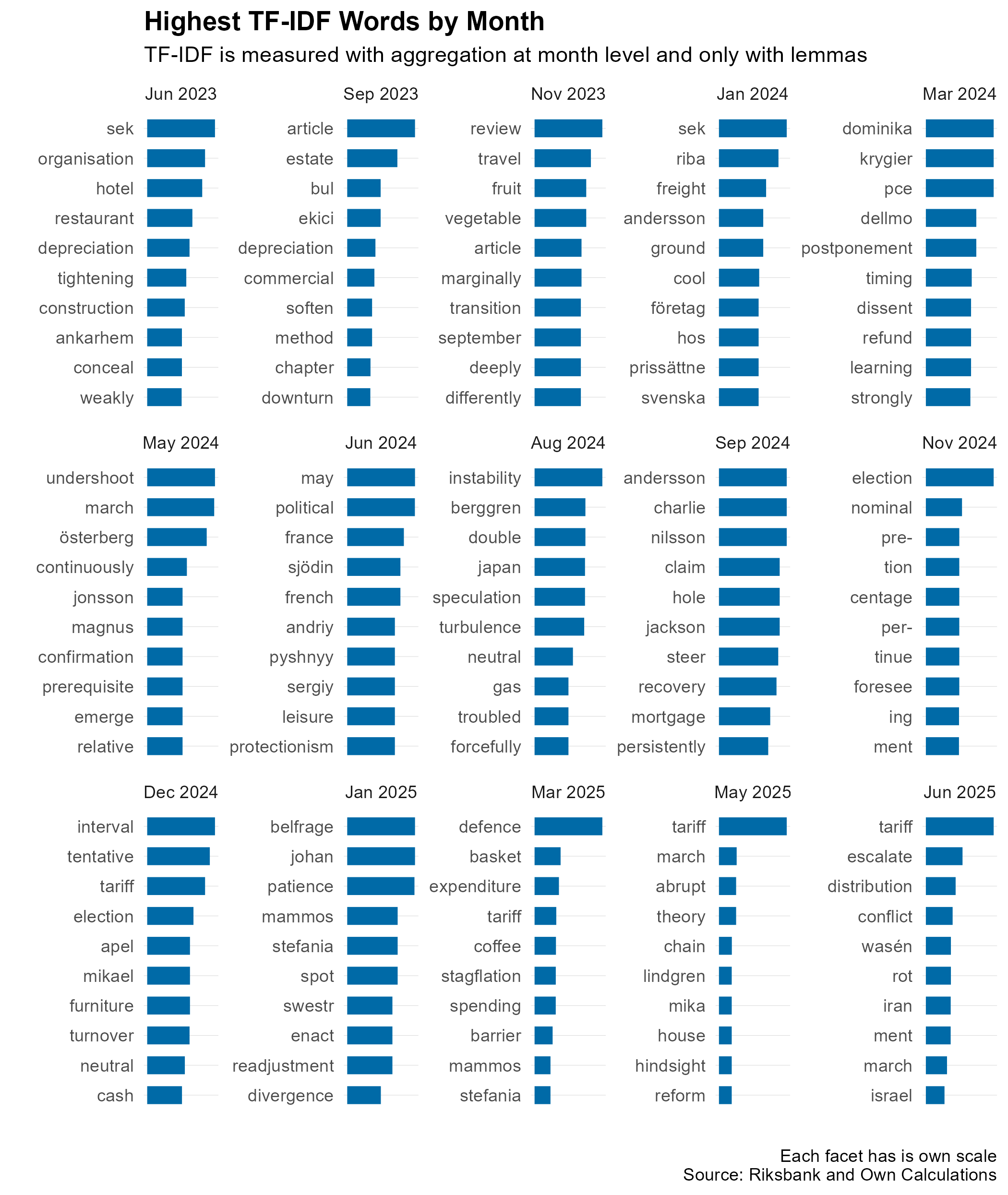
The graph above does the same analysis as the previous one, but now each month is considered an unique document. I select minutes from the last 24 months, to see what the Riksbank has been focusing on lately.

In 2025, following Trump’s election, tariffs have been on the spotlight. On the last minute, though, the Israel-Iran war was strongly mentioned too. Europe moving towards larger defence spending has also been noted in March, as well as higher coffee prices and stagflation risk amidst a trade war. On the end of 2024, the Jackson Hole forum was also mentioned, as well as the US election.

In August 2024, the stock market drop in Japan, following a BOJ surprise hike, expectations of FED rate cuts and a yen appreciation, was highlighted in Riksbank minutes. The expectations of under 2% CPIF inflation in late 2024 were noted in May, as “undershoot” was notoriously mentioned, as inflation lost momentum and base period effect would become supportive of low year-over-year inflation in the second semester. French elections also received attention in June.

Finally, in the second semester of 2023, the vulnerability of the Swedish Krone was the focus of Riksbank minutes, as “sek” and “depreciation” reached high scores in July and October.

Latent Dirichlet Allocation

The Latent Dirichlet Allocation model is an unsupervised machine learning algorithm that, given an arbitrary k amount of topics, calculates the probability of a document being generated by each of them. Using the pre-determined Document Term Matrix, we run the algorithm through a Gibbs Sampler, considering 8 topics. The ten thousand iterations take a while to run.

model <- LDA(DTM, method="Gibbs", k = 8, control = list(iter = 10000))


colnames_holder <- apply(terms(model, 7),2, paste, collapse = " ") %>%
  str_to_title()

topics <- tidy(model, matrix = "beta")
documents <- tidy(model, matrix = "gamma")

db_graph <- full_join(data_lda, documents %>% rename("doc_id" = "document")) %>%
  mutate(date = as_date(as.yearmon(date))) %>%
  reframe(cont = 100*mean(gamma), .by = c(date, topic)) %>%
  na.omit %>%
  pivot_wider(names_from = topic, values_from = cont) %>%
  rename_with(~c("date", colnames_holder)) %>%
  pivot_longer(-date, names_to = "topic", values_to = "cont") %>%
  group_by(topic) %>%
  filter(year(date) >= 2001) %>%
  mutate(topic = factor(topic))

g7_1 <- ggplot(data = db_graph) +
  geom_line(aes(x = date, y = cont), colour = "#006AA7") +
  facet_wrap(~topic, scales = "free", nrow = 2, label = as_labeller(label_wrap(40))) +
  theme_minimal() + xlab("") + ylab("") +
  scale_y_continuous(breaks = pretty_breaks(n=10)) +
  scale_x_date(labels = date_format("%b %y"),
               breaks = seq.Date(from=min(db_graph$date),
                                 to=max(db_graph$date),
                                 length.out=13),
               expand = expansion(mult = c(0.01,0.05))) +
  labs(title="Topic Distribution Across Time",
       subtitle="%, Latent Dirichlet Allocation Model",
       caption = "Number consists of mean probability of sentences being generated by topic
Words highlighted are the most likely words to be generated by topic, in order
Source: Riksbank and Own Calculations") +
  theme(panel.grid.major.x = element_blank(),
        panel.grid.minor.x = element_blank(),
        panel.grid.major.y = element_line(colour="lightgray", size=0.1),
        panel.grid.minor.y = element_line(colour="lightgray", size=0.1),
        axis.text.x = element_text(angle = 90, vjust = 0.5, hjust=1),
        plot.title=element_text(face="bold"),
        legend.title=element_blank(),
        legend.key.size = unit(0.8, "cm")) +
  theme(legend.box = "horizontal")+
  guides(col = guide_legend(direction = "horizontal"),
         fill = guide_legend(direction = "horizontal"),
         shape = guide_legend(direction = "horizontal")) +
  theme(legend.position=c(1, 1.015),
        legend.justification="right",
        plot.title = element_text(vjust = 1.5),
        plot.subtitle = element_text(vjust = 3.75))


db_graph <- full_join(data_lda, documents %>% rename("doc_id" = "document")) %>%
  mutate(date = as_date(as.yearmon(date))) %>%
  reframe(cont = 100*mean(gamma), .by = c(date, topic)) %>%
  na.omit %>%
  pivot_wider(names_from = topic, values_from = cont) %>%
  rename_with(~c("date", colnames_holder)) %>%
  pivot_longer(-date, names_to = "topic", values_to = "cont") %>%
  group_by(topic) %>%
  filter(year(date) >= 2019) %>%
  mutate(topic = factor(topic))

g7_2 <- ggplot(data = db_graph) +
  geom_line(aes(x = date, y = cont), colour = "#006AA7") +
  facet_wrap(~topic, nrow = 2, label = as_labeller(label_wrap(40))) +
  theme_minimal() + xlab("") + ylab("") +
  scale_y_continuous(breaks = pretty_breaks(n=10)) +
  scale_x_date(labels = date_format("%b %y"),
               breaks = seq.Date(from=min(db_graph$date),
                                 to=max(db_graph$date),
                                 length.out=13),
               expand = expansion(mult = c(0.01,0.05))) +
  labs(title="Topic Distribution Across Time, Zoomed",
       subtitle="%, Latent Dirichlet Allocation Model",
       caption = "Number consists of mean probability of sentences being generated by topic
Words highlighted are the most likely words to be generated by topic, in order
Source: Riksbank and Own Calculations") +
  theme(panel.grid.major.x = element_blank(),
        panel.grid.minor.x = element_blank(),
        panel.grid.major.y = element_line(colour="lightgray", size=0.1),
        panel.grid.minor.y = element_line(colour="lightgray", size=0.1),
        axis.text.x = element_text(angle = 90, vjust = 0.5, hjust=1),
        plot.title=element_text(face="bold"),
        legend.title=element_blank(),
        legend.key.size = unit(0.8, "cm")) +
  theme(legend.box = "horizontal")+
  guides(col = guide_legend(direction = "horizontal"),
         fill = guide_legend(direction = "horizontal"),
         shape = guide_legend(direction = "horizontal")) +
  theme(legend.position=c(1, 1.015),
        legend.justification="right",
        plot.title = element_text(vjust = 1.5),
        plot.subtitle = element_text(vjust = 3.75))

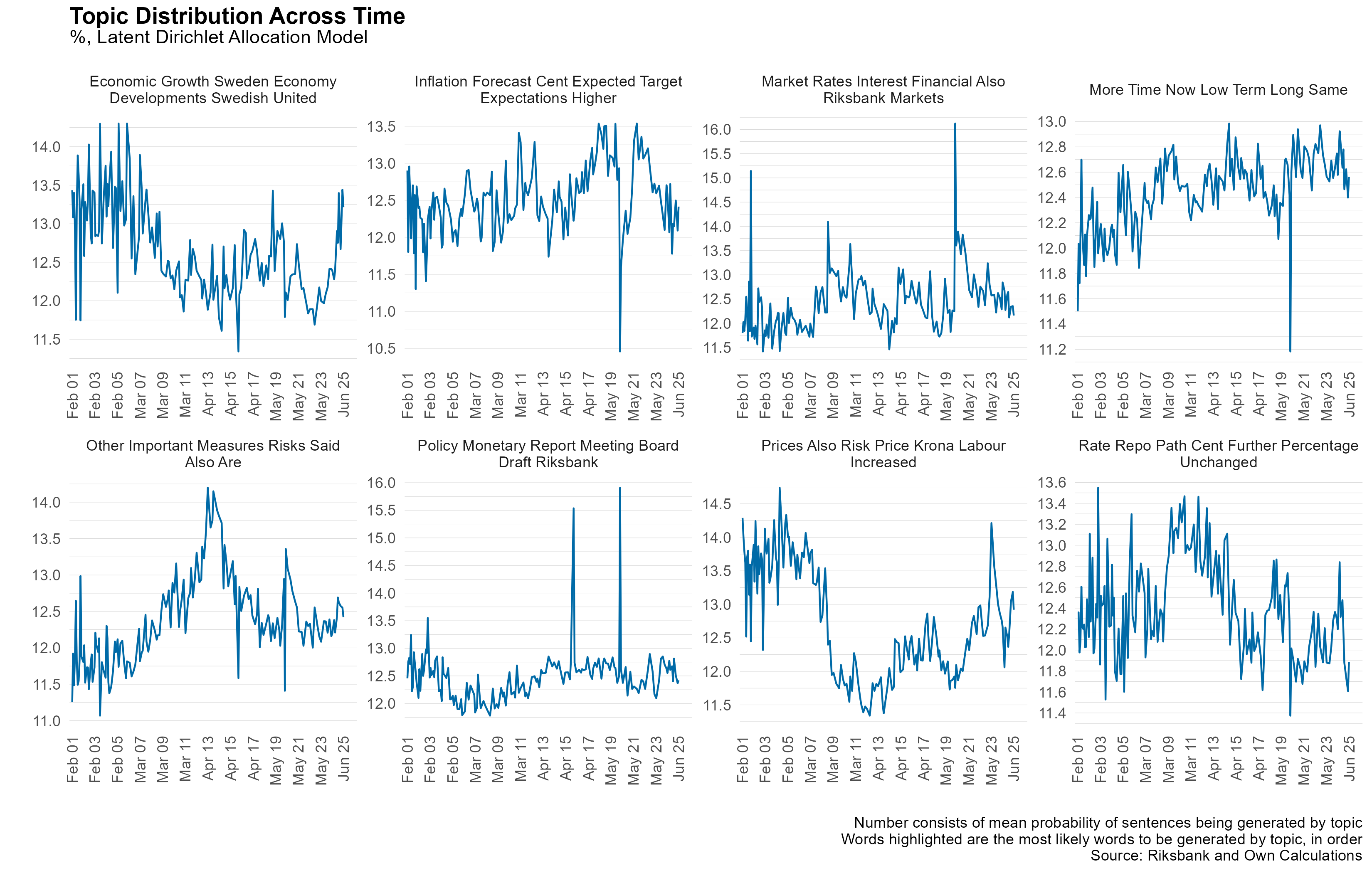
g7_1

g7_2

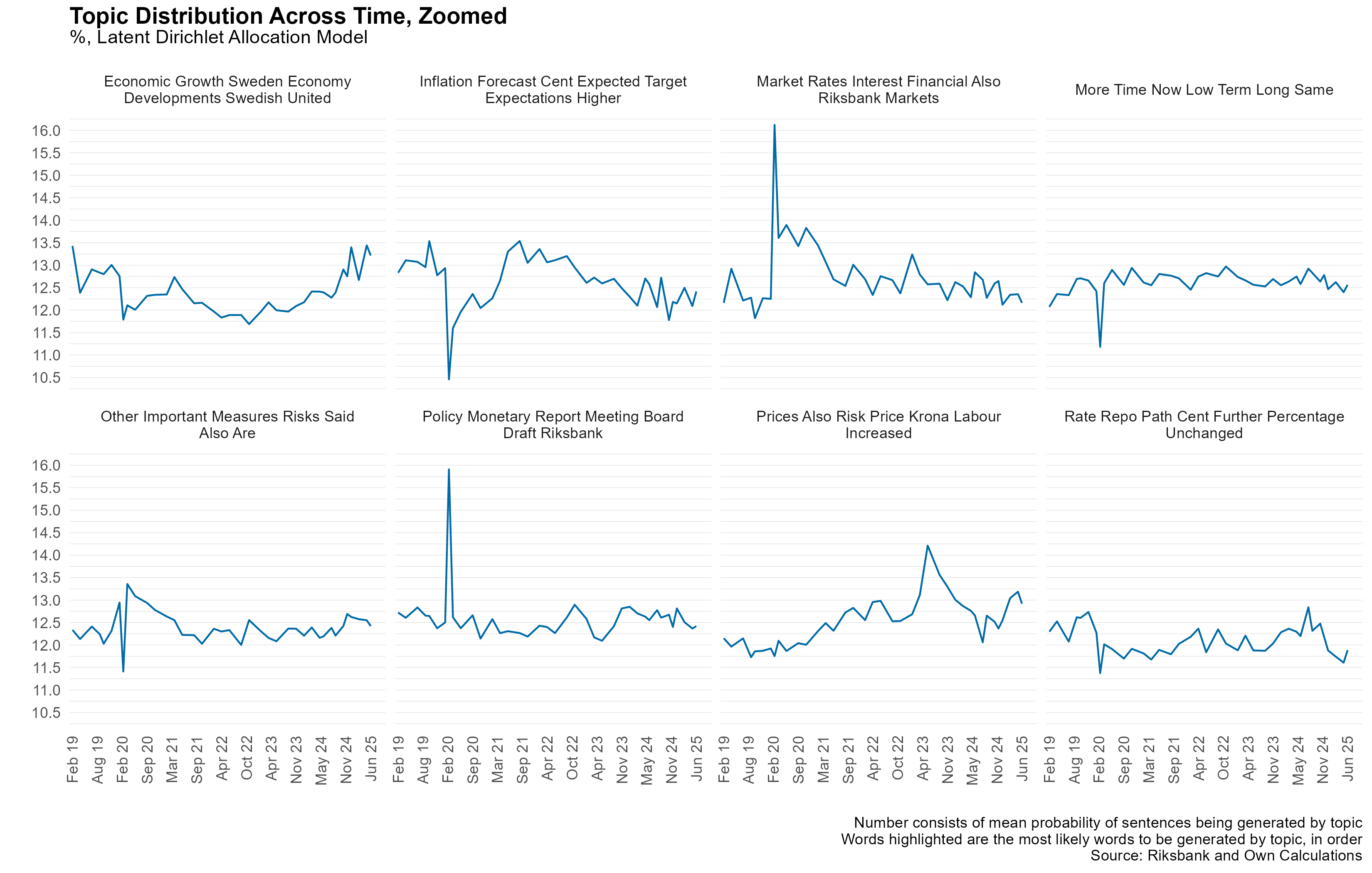
These two graphs show the evolution of mean probability of a sentence “belonging” to each topic in each minute. The words selected are the seven more frequent words in each of the topics. It is important to display them to shed some light on what the topics are actually about.

Unfortunately they do not tell a clear story. It is worth noting the rise in the sixth topic, which seems to be related to higher prices, in the post-pandemic inflationaty spike.

db_graph <- topics %>%
  group_by(topic) %>%
  arrange(beta) %>%
  slice_tail(n = 20)

g8 <- ggplot(db_graph, aes(label = term), colour = "#006AA7") +
  geom_text_wordcloud(aes(size = beta)) +
  facet_wrap(~topic) +
  theme_minimal() +
  labs(title="20 Most Likely Words by Topic",
       subtitle="
         Latent Dirichlet Allocation Model (Machine Learning)
         Size is equivalent to likelihood",
       caption="Source: Riksbank and Own Calculations") +
  theme(panel.grid = element_line(colour="lightgray", size=0.1),
        axis.text.x = element_text(vjust = 0.5, hjust=1,
                                   angle=90),
        plot.title=element_text(face="bold"),
        legend.title=element_blank(),
        legend.key.size = unit(0.5, "cm"))

g8

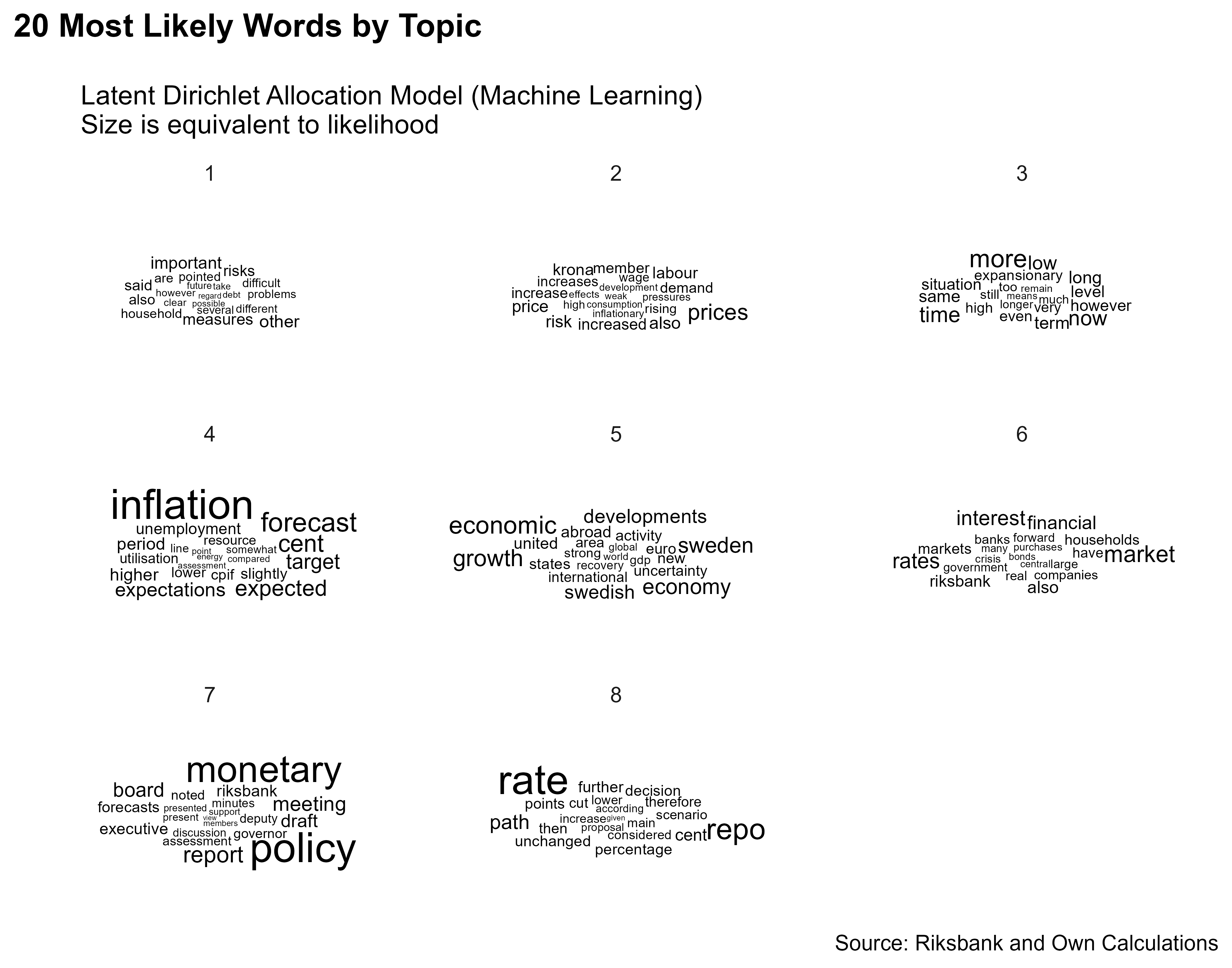
The graph above aggregates the twenty most likely words to be generated by each topic in word clouds. The bigger the word, the highest the probability.

Modelling

I’ve explored the content of the minutes to tell a story about the present and the past of the Swedish economy. But can this data help explain future decisions?

To answer that, I run an Ordered Probit Model to find if Minutes sentiment can help explain moves in the policy rate.

Data Preprocessing

To start, it is necessary to download the policy rate data from the Riksbank’s API. I then complete, adding days in which there is no banking activity and carrying the latest observation before for these dates.

resp <- request("https://api.riksbank.se/swea/v1/Observations/SECBREPOEFF/2000-01-01") %>%
  req_headers(
    Accept = "application/json"
  ) %>%
  req_perform()

pr <- resp %>% 
  resp_body_json() %>% 
  map(., ~as.data.frame(.x)) %>% 
  bind_rows %>% 
  mutate(date = as_date(date)) %>%
  complete(date = seq(min(date), max(date), by = "day")) %>%
  mutate(value = na.locf(value, na.rm = F))

To bind the policy rate data with the sentiment from the minutes, it is crucial to be careful. The policy rate in he Riksbank’s data does not change in the day that the decision is taken, but rather on the day it is effectively valid. So, to correctly match the date that meetings took place with the respective policy rate decided, I carry the number of the minute and the sentiment of it forward. Then, for all observations relating to the same minute, I change the date to the first (which is the actual data the the board opted or a change in the policy rate, it has also effectively changed and there is no mismatch.

pr_sentiment <- data_sentiment_bert %>%
  ungroup %>%
  filter(year(date) >= 2000) %>%  

  mutate(label = case_when(label == "Negative" ~ -1,
                           label == "Neutral" ~ 0,
                           label == "Positive" ~ 1)) %>% 
  reframe(sentiment = mean(score*label),
          .by = date) %>% 
  mutate(n = row_number()) %>% 
  full_join(pr) %>% 
  arrange(date) %>%
  mutate(n = na.locf(n, na.rm = F),
         sentiment = na.locf(sentiment, na.rm = F)) %>%
  na.omit %>%
  mutate(date = first(date), .by = n) %>%
  group_by(date) %>%
  slice_tail(n=1) %>% 
  ungroup %>% 
  mutate(sentiment = scale(sentiment)[,1]) %>% 
  mutate(value = value - lag(value)) %>% 
  na.omit %>% 
  mutate(policy = case_when(value == 0 ~ "hold",
                            value < 0 ~ "cut", 
                            value > 0 ~ "hike"),
         policy = factor(policy, levels = c("cut", "hold", "hike"))) 

Ordered Probit Model

Now, I can run the model. I use MASS::polr to run the Ordered Probit Model. The option for this model is inspired by Apel, Grimaldi (2012). They do a similar job, constructing an index of hawkishness/doviness on the Riksbank minutes and testing if it helps explain changes in the rate. Inspired by them, I define three levels: cut, hold and hike. I use the sentiment calculed with the FinBERT model and the lag of the decision as regressors.

library(MASS)

model_probit <- polr(policy ~ lag(sentiment) + lag(policy), data = pr_sentiment, 
                     method = "probit",   
                     Hess   = TRUE)

ctable <- coef(summary(model_probit))
p_values <- pnorm(abs(ctable[,"t value"]), lower.tail = FALSE)*2
cbind(ctable, "p value" = p_values)

##                      Value Std. Error   t value      p value
## lag(sentiment)   0.2427377 0.09518852  2.550074 1.077001e-02
## lag(policy)hold  0.7184828 0.25709163  2.794656 5.195491e-03
## lag(policy)hike  2.1898508 0.34576352  6.333377 2.398524e-10
## cut|hold        -0.2658864 0.22407621 -1.186589 2.353897e-01
## hold|hike        1.9840095 0.27198755  7.294487 2.997998e-13

These results tell us that an increase in one standard deviation of sentiment in the previous minute increases the latent score by 0.243. The value is statistically significant, as the p-value is approximately 0.01.

The sign of the impact is in line with the expected: when the economy is doing well and mood is good, the Bank is more likely to hike, and when the economy is doing bad and mood is down, the Bank is more likely to cut. As the sample starts in 2000, the only period in which the Riksbank faced high and persistent inflation was after the pandemic. For an economy with low inflation rates, low potential growth and high exposure to the global economy, it makes sense that the Central Bank would be more active in stabilizing output, rather than inflation. Therefore, the reaction to overall sentiment is reasonable.

The lag of policy being statistically significant for hold indicates that a previous hold reduces probability of cuts. The 2.19 value for a previous hike by itself puts the latent score above the hold|hike threshold, indicating that the Riksbank rarely hikes and stops or reverse course in the following meeting. The cut|hold threshold not being statistically significant indicates that, in constrast to hikes, cuts and holds are not easily distinguishable.

Now, I add the CPIF inflation and the monthly GDP indicator, to check if the significance of the sentiment still holds. Unfortunately, I don’t have the information on when this data was released, but we regress them lagged, so this should not be a problem, as the Bank probably had the previous month information by the time of the meeting.

payload <- '{
  "query": [
    {
      "code": "ContentsCode",
      "selection": {
        "filter": "item",
        "values": "000005HR"
      }
    }
  ],
  "response": {
    "format": "json"
  }
}'

cpif <- pxweb::pxweb_get_data(url = "https://api.scb.se/OV0104/v1/doris/en/ssd/START/PR/PR0101/PR0101G/KPIF",
                      query = payload) %>% 
  rename_with(~c("date", "cpif")) %>% 
  mutate(date = ym(gsub("M", "-", date))) %>% 
  mutate(cpif = 100*(cpif/lag(cpif)-1))


payload = '{
  "query": [
    {
      "code": "ContentsCode",
      "selection": {
        "filter": "item",
        "values": [
          "000000X3"
        ]
      }
    }
  ],
  "response": {
    "format": "json"
  }
}'

gdp <- pxweb::pxweb_get_data(url = "https://api.scb.se/OV0104/v1/doris/en/ssd/START/NR/NR9999/NR9999A/NR9999ENS2010BNPIndN",
                      query = payload) %>% 
  dplyr::select(-1) %>% 
  rename_with(~c("date", "gdp")) %>% 
  mutate(date = ym(gsub("M", "-", date))) %>% 
  mutate(gdp = 100*(gdp/lag(gdp)-1))

pr_sentiment_extended <- pr_sentiment %>% 
  mutate(date = as_date(as.yearmon(date))) %>% 
  left_join(cpif) %>% 
  left_join(gdp) %>% 
  na.omit

model_probit <- polr(policy ~ lag(sentiment) + lag(policy) + lag(gdp) + lag(cpif), data = pr_sentiment_extended, 
                     method = "probit",   
                     Hess   = TRUE)       

ctable <- coef(summary(model_probit))
p_values <- pnorm(abs(ctable[,"t value"]), lower.tail = FALSE)*2
cbind(ctable, "p value" = p_values)

##                       Value Std. Error    t value      p value
## lag(sentiment)   0.21552297 0.09754733  2.2094195 2.714548e-02
## lag(policy)hold  0.76278938 0.26071007  2.9258148 3.435554e-03
## lag(policy)hike  2.16588748 0.34898682  6.2062158 5.427565e-10
## lag(gdp)         0.01029778 0.07069813  0.1456585 8.841910e-01
## lag(cpif)        0.42231785 0.26081480  1.6192250 1.053989e-01
## cut|hold        -0.16968113 0.23215926 -0.7308825 4.648509e-01
## hold|hike        2.10706879 0.28262518  7.4553470 8.963158e-14

The value for the coefficient of sentiment barely changes and the p-value increases to 0.027, indicating that the variable is still statistically significant at 5%. GDP and CPIF do not impact the policy decision in a statistically significant way.

Conclusion

I conducted an extense text analysis on the minutes of the Riksbank, using a wide variety of techniques, ranging from word counting, to machine-learning and AI algorithms. The graphs generated help tell the story of the Swedish economy in the last three decades.

Moreover, in the last section, I show that the minutes are also helpful in preventing insights into the future, as the sentiment on the previous minute helps predict policy rate moves at the next meeting.