Forecasting UK imports data with Elastic Net models in a Tidymodels pipeline

Table of Contents

• Introduction
• Setup
• Data Collection
  • National Highways Traffic
  • ONS Shipping Data
  • Debit Card Spending
  • Terms of Trade
  • Imports & Industrial Production
  • Global Economic Conditions
  • Real Effective Exchange Rate
• Modeling
  • Data Preprocessing
  • Time Series Cross Validation
  • Elastic Net Tuning
  • Baseline AR(2) Model
  • Forecast Comparison
  • Adaptive Elastic Net
  • Regularization Path
• Conclusion

---

Introduction

This report presents a forecasting model for UK monthly goods imports using the Elastic Net method within the tidymodels framework. The model includes high frequency data from different sources on ships arrival, traffic, economic activity and other financial and macroeconomic indicators

The goal is to evaluate the forecast performance of multiple Elastic Net models compared to a baseline autoregressive model and investigate the regularization path of predictors.

---

Setup

Note: All required packages are loaded below. Messages and warnings are suppressed for clarity.

# General data wrangling and visualization
library(tidyverse)
library(zoo)
library(lubridate)

# Modeling and forecasting
library(tidymodels)
library(glmnet)
library(timetk)
library(urca)

# API and web scraping
library(httr2)
library(rvest)
library(readxl)
library(vroom)

# Time formatting and external data
library(ISOweek)
library(onsr)

# Set locale to English for month names
invisible(Sys.setlocale("LC_TIME", "C"))

---

Data Collection

National Highways Traffic

We start by collecting traffic data from the UK’s National Highways API. We select two key sites:

• A14/2040A: Access to Felixstowe Port
• M27/9132B: Access to Southampton Port

The API provides monthly data on total vehicle flow and the proportion of large vehicles registered at each site.

# Step 1: Request site metadata from the National Highways API
url <- "https://webtris.nationalhighways.co.uk/api/v1/sites"

request <- request(url) %>% 
  req_headers(Accept = "application/json") %>% 
  req_perform() 

# Step 2: Parse response and consolidate all sites into a single dataframe
all_sites <- request %>% 
  resp_body_json %>% 
  .[[2]] %>% 
  map(., ~as.data.frame(.x)) %>% 
  bind_rows

# Step 3: Filter for the selected MIDAS sites
sites_filtered <- all_sites %>% 
  filter(Status == "Active" & grepl("A14/2040A|M27/9132B", Name))

# Step 4: Construct API URL to pull monthly data from the selected sites
url <- paste0(
  "https://webtris.nationalhighways.co.uk/api/v1/reports/01012016/to/",
  gsub("-", "", format(Sys.Date(), "%d%m%Y")),
  "/monthly?sites=", paste(sites_filtered$Id, collapse = ","),
  "&page=1&page_size=30000"
)

request <- request(url) %>% 
  req_headers(Accept = "application/json") %>% 
  req_perform()

# Step 5: Parse monthly data, reshape, and filter out incomplete rows
df_traffic <- request %>% 
  resp_body_json %>% 
  .$MonthCollection %>% 
  map(., ~data.frame(
    date = .x$Month,
    id = .x$SiteId,
    Flow = .x$`Summary Aggregation`$ADT24Hour,
    Heavy_Pct = .x$`Summary Aggregation`$ADT24HourLargeVehicle
  )) %>% 
  bind_rows %>% 
  mutate(date = my(date)) %>% 
  pivot_wider(names_from = id, values_from = c(Flow, Heavy_Pct)) %>% 
  filter(row_number() > max(row_number()[if_any(everything(), is.na)]))

df_traffic %>% head(5)

## # A tibble: 5 × 5
##   date       Flow_2900 Flow_3840 Heavy_Pct_2900 Heavy_Pct_3840
##   <date>     <chr>     <chr>     <chr>          <chr>         
## 1 2018-05-01 19349     62909     17.6           6.2           
## 2 2018-06-01 19563     64608     17.4           6.4           
## 3 2018-07-01 20002     65478     16.3           6.3           
## 4 2018-08-01 19866     66797     17.1           6.3           
## 5 2018-09-01 18760     59309     17.2           6.5

ONS Shipping Data

We then collect ship visit data from the UK’s Office for National Statistics using the onsr package. This includes monthly counts of cargo and tanker ship visits aggregated across all UK ports.

The dataset includes weekly-level observations in ISO format. Since our analysis is monthly, we use the end-of-week dates to assign each observation to a month and then compute the monthly mean. This is an approximation, as some weeks span two months and cause slight misalignment.

# Step 1: Download shipping activity data from ONS API
df_ports_raw <- ons_get("faster-indicators-shipping-data")

# Step 2: Filter relevant ship types and parse week-year strings into monthly dates
df_ports <- df_ports_raw %>% 
  filter(Port == "All of UK", ShipAndVisitType == "Cargo and tanker visits") %>% 
  select(Time, Week, v4_1) %>% 
  mutate(Week = gsub("Week ", "", Week),
        date = sprintf("%d-W%02d", as.numeric(Time), as.numeric(Week))) %>% 
  mutate(date = ISOweek2date(paste0(date,"-7"))) %>% 
  mutate(date = as_date(as.yearmon(date))) %>% 
  na.omit %>% 
  reframe(CargoTankerVisits = mean(v4_1, na.rm = T),
          .by = date) %>% 
  arrange(date)

df_ports %>% head(5)

## # A tibble: 5 × 2
##   date       CargoTankerVisits
##   <date>                 <dbl>
## 1 2019-01-01              516.
## 2 2019-02-01              584.
## 3 2019-03-01              581.
## 4 2019-04-01              543.
## 5 2019-05-01              531

Debit Card Spending

Most ONS data series relevant to forecasting the trade balance are not available via API. Therefore, we resort to webscraping. The general process is as follows: we access the ONS webpage, locate the most recent Excel file using the rvest package, download the file to a temporary location, and read in the desired sheet. As a first example, we collect debit card spending, a high-frequency indicator of domestic demand and economic activity.

The latest edition will always be the first shown on the page. We create a temporary file to store the downloaded spreadsheet and use download.file() with mode = “wb” (workbook). Finally, we read Table 4 from the sheet using the readxl package, as it contains the monthly aggregated totals.

# Step 1: Define URL of debit card spending dataset from ONS
url = "https://www.ons.gov.uk/economy/economicoutputandproductivity/output/datasets/revolutspendingondebitcards"

# Step 2: Scrape all available Excel sheet links using rvest
excel_sheets <- read_html(url) %>% 
  html_elements("a") %>% 
  html_attr("href") %>% 
  .[grepl(".xls", .)]

# Step 3: Download the latest available file (first on the page)
xls_link <- excel_sheets[1]
p1f <- tempfile()
download.file(paste("ons.gov.uk", xls_link, sep=""), p1f, mode = "wb")

# Step 4: Read relevant table from Excel file (Table 4, aggregated data)
df_card_raw <- read_excel(p1f, sheet = "Table 4", skip = 6)
invisible(file.remove(p1f))

# Step 5: Clean and format data into final monthly structure
df_card <- df_card_raw %>% 
  select(Date, Total) %>% 
  rename_with(~c("date", "CardSpending")) %>% 
  mutate(date = my(date))

df_card %>% head(5)

## # A tibble: 5 × 2
##   date       CardSpending
##   <date>            <dbl>
## 1 2020-01-01         66.8
## 2 2020-02-01         66.1
## 3 2020-03-01         48.9
## 4 2020-04-01         27.5
## 5 2020-05-01         35.0

Terms of Trade

Next, we collect terms of trade data. This process mirrors earlier steps: we locate the most recent Excel file link using the rvest package, download it to a temporary file, and read in the relevant sheet. This dataset provides monthly indices that reflect the ratio of export to import prices, a key macroeconomic driver of trade dynamics.

# Step 1: Define the URL of the ONS terms of trade dataset
url = "https://www.ons.gov.uk/economy/nationalaccounts/balanceofpayments/timeseries/ctsl/mret"

# Step 2: Scrape Excel sheet links from the page
excel_sheets <- read_html(url) %>% 
  html_elements("a") %>% 
  html_attr("href") %>% 
  .[grepl(".xls", .)]

# Step 3: Download the most recent file (top of the list)
xls_link <- excel_sheets[1]
p1f <- tempfile()
download.file(paste("ons.gov.uk", xls_link, sep=""), p1f, mode = "wb")

# Step 4: Read data from the "data" sheet, skipping metadata rows
df_tot_raw <- read_excel(p1f, sheet = "data", skip = 7)
invisible(file.remove(p1f))

# Step 5: Parse and format data for use in the model
df_tot <- df_tot_raw %>% 
  rename_with(~c("date", "TOT")) %>% 
  filter(grepl("([A-Za-z].*){3,}", date)) %>% 
  mutate(date = ym(date))

df_tot %>% head(5)

## # A tibble: 5 × 2
##   date         TOT
##   <date>     <dbl>
## 1 1997-01-01  88.3
## 2 1997-02-01  87.9
## 3 1997-03-01  88  
## 4 1997-04-01  88  
## 5 1997-05-01  87.3

Imports & Industrial Production

We then retrieve the UK’s monthly imports data (our dependent variable) and industrial production index. These two datasets are usually released together, although in different pages.

# Step 1: Define URL for UK goods trade balance dataset
url = "https://www.ons.gov.uk/economy/nationalaccounts/balanceofpayments/datasets/tradeingoodsmretsallbopeu2013timeseriesspreadsheet"

# Step 2: Scrape link to latest Excel file
xls_link <- read_html(url) %>% 
  html_elements("a") %>% 
  html_attr("href") %>% 
  .[grepl(".xls", .)]

# Step 3: Download and read the sheet containing import data
p1f <- tempfile()
download.file(paste("ons.gov.uk", xls_link, sep=""), p1f, mode = "wb")

# Step 4: Extract raw data from Excel
df_imports_raw <- read_excel(p1f, sheet = "data", skip = 1)
invisible(file.remove(p1f))

# Step 5: Clean and select monthly import data
df_imports <- df_imports_raw %>% 
  select(CDID, BOKH) %>% 
  rename_with(~c("date", "Imports")) %>% 
  filter(grepl("([A-Za-z].*){3,}", date)) %>% 
  mutate(date = ym(date)) %>% 
  na.omit

# Step 6: Fetch industrial production data from ONS
url = "https://www.ons.gov.uk/economy/economicoutputandproductivity/output/datasets/indexofproduction"

# Step 7: Scrape link to latest Excel file
xls_link <- read_html(url) %>% 
  html_elements("a") %>% 
  html_attr("href") %>% 
  .[grepl(".xls", .)]

# Step 8: Download and extract industrial production time series
p1f <- tempfile()
download.file(paste("ons.gov.uk", xls_link, sep=""), p1f, mode = "wb")

df_ip_raw <- read_excel(p1f, sheet = "data", skip = 1)
invisible(file.remove(p1f))

# Step 9: Clean and convert industrial production to monthly format
df_ip <- df_ip_raw %>% 
  select(CDID, K222) %>% 
  rename_with(~c("date", "IP")) %>% 
  filter(grepl("([A-Za-z].*){3,}", date)) %>% 
  mutate(date = ym(date)) %>% 
  na.omit %>% 
  mutate(IP = as.numeric(IP))

df_ip %>% head(5)

## # A tibble: 5 × 2
##   date          IP
##   <date>     <dbl>
## 1 1948-01-01  28  
## 2 1948-02-01  28  
## 3 1948-03-01  28  
## 4 1948-04-01  28  
## 5 1948-05-01  28.1

Global Economic Conditions

We also include a proxy for global demand: the Global Economic Conditions Indicator (GECON) from Baumeister, Korobilis, & Lee (2022). The time series is publicly available at this repository.

url = "https://drive.google.com/uc?export=download&id=1-xGp5-PvgjoAcDQuw09nq4Kgoj16hqsu"

p1f <- tempfile()
download.file(url, p1f, mode = "wb")

# Load and clean the GECON data
df_gecon_raw <- read_excel(p1f)
invisible(file.remove(p1f))

df_gecon <- df_gecon_raw %>% 
  select(`...1`, `Global Economic Conditions Indicator`) %>% 
  rename_with(~c("date", "GECON")) %>% 
  mutate(date = ym(date))

df_gecon %>% head(5)

## # A tibble: 5 × 2
##   date         GECON
##   <date>       <dbl>
## 1 1973-02-01  0.594 
## 2 1973-03-01  0.393 
## 3 1973-04-01 -0.118 
## 4 1973-05-01  0.0939
## 5 1973-06-01  0.0499

Real Effective Exchange Rate

To control for external price competitiveness, we include the UK’s broad real effective exchange rate (REER), fetched directly from the Bank for International Settlements API.

df_reer_raw <- vroom("https://stats.bis.org/api/v2/data/dataflow/BIS/WS_EER/1.0/D.N.B.GB?format=csv")

# Parse and average the REER data to monthly
df_reer <- df_reer_raw %>% 
  select(TIME_PERIOD, OBS_VALUE) %>% 
  rename_with(~c("date", "REER")) %>% 
  mutate(date = as_date(as.yearmon(date))) %>% 
  reframe(REER = mean(REER, na.rm = TRUE), .by = date)

df_reer %>% head(5)

## # A tibble: 5 × 2
##   date        REER
##   <date>     <dbl>
## 1 1996-04-01  97.6
## 2 1996-05-01  98.5
## 3 1996-06-01 100. 
## 4 1996-07-01 100. 
## 5 1996-08-01  99.4

Modelling

Elastic Net Regression

The Elastic Net (Zou & Hastie, 2005) is a regularized regression method that linearly combines the penalties of the Lasso (\(\ell_1\)) and Ridge (\(\ell_2\)) regressions. It addresses two key limitations of the Lasso:

1. Its tendency to select only one variable from a group of correlated predictors,
2. Its instability in high-dimensional settings.

By introducing a mixing parameter, the Elastic Net allows the model to balance variable selection and coefficient shrinkage, making it particularly effective when dealing with multicollinearity and large feature spaces. As we do not know which variables are relevant to explain UK imports ex-ante, this is an interesting approach.

Mathematically, it solves the following optimization problem:

\[\hat{\beta} = \arg\min_{\beta} \left\{ \frac{1}{2n} \| y - X\beta \|_2^2 + \lambda \left( \alpha \|\beta\|_1 + \frac{1 - \alpha}{2} \|\beta\|_2^2 \right) \right\}\]

Where:

• \(\lambda\) controls the overall strength of regularization
• \(\alpha \in [0, 1]\) determines the trade-off between Lasso \(( \alpha = 1 )\) and Ridge \(( \alpha = 0 )\)

---

Data Preprocessing

We join all the data and do necessary transformations. Almost all variables are in percentage change, apart from the heavy vehicles percentages, in first differences, and the GECON which is a diffusion index with mean 0. Industrial production and terms of trade enter the model lagged due to release mismatch.

dfs <- list(df_imports, df_card, df_gecon, df_ip, df_ports, df_reer, df_tot, df_traffic)
df_final <- reduce(dfs, full_join) %>% 
  arrange(date) %>% 
  mutate(across(-date, ~as.numeric(.x))) %>% 
  mutate(across(contains("Heavy"), ~.x-lag(.x))) %>% # Variables containing heavy percentage are in 1st difference
  mutate(across(-c(date, contains("Heavy"), GECON), ~100*(.x/lag(.x)-1))) %>% # Other variables are in percentage difference, while GECON is already stationary and does not need transformation
  mutate(across(c(IP, TOT), ~lag(.x))) %>% # Industrial production and Terms of Trade must be lagged due to late release
  mutate(Imports_lag1 = lag(Imports,1),
         Imports_lag2 = lag(Imports,2)) %>% 
  na.omit

df_final %>% tail(5)

## # A tibble: 5 × 14
##   date       Imports CardSpending   GECON     IP CargoTankerVisits   REER
##   <date>       <dbl>        <dbl>   <dbl>  <dbl>             <dbl>  <dbl>
## 1 2024-10-01   7.62       -0.0587  0.194  -0.204            -0.178  0.182
## 2 2024-11-01   1.36       -2.46    0.177  -0.714            -2.16  -0.390
## 3 2024-12-01  -2.91        6.49    0.172  -0.308            -9.77   0.309
## 4 2025-01-01   0.773      -8.66   -0.111   1.03             -0.692 -1.54 
## 5 2025-02-01   5.22       -5.79   -0.0355 -0.510            10.3    0.864
## # ℹ 7 more variables: TOT <dbl>, Flow_2900 <dbl>, Flow_3840 <dbl>,
## #   Heavy_Pct_2900 <dbl>, Heavy_Pct_3840 <dbl>, Imports_lag1 <dbl>,
## #   Imports_lag2 <dbl>

The Augmented Dickey-Fuller test rejects presence of unit root for all variables, indicating no sign of non-stationarity.

df_final %>%
  select(-date) %>%
  map(~ ur.df(.x, type = "drift", selectlags = "AIC")) %>%
  map_df(~ {
    test_stat <- .x@teststat[1]
    tibble(
      `ADF Test Statistic` = round(test_stat, 3)
    )
  }, .id = "Variable") %>% 
  head(15)

## # A tibble: 13 × 2
##    Variable          `ADF Test Statistic`
##    <chr>                            <dbl>
##  1 Imports                          -6.10
##  2 CardSpending                     -5.84
##  3 GECON                            -6.91
##  4 IP                               -7.56
##  5 CargoTankerVisits                -8.07
##  6 REER                             -6.00
##  7 TOT                              -7.05
##  8 Flow_2900                        -6.21
##  9 Flow_3840                        -6.89
## 10 Heavy_Pct_2900                   -7.26
## 11 Heavy_Pct_3840                   -7.91
## 12 Imports_lag1                     -6.07
## 13 Imports_lag2                     -6.06

---

Time Series Cross Validation

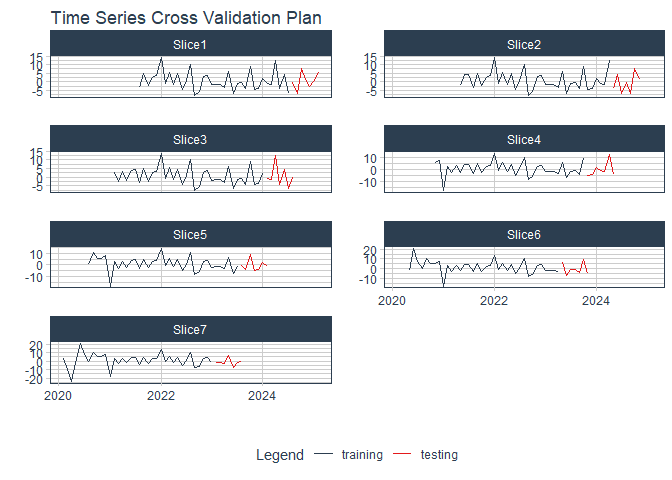
We implement a time-series cross-validation scheme using the timetk package to assess model performance on rolling forecasting origins. Specifically:

• A sliding window (initial = "3 years") is used to train the model on a fixed-size training set.
• Each resample forecasts the next 7 months (assess = 7).
• Windows advance by 3 months (skip = 3) with no cumulative growth (cumulative = FALSE).

We also create a final training/test split for out-of-sample evaluation using the last 7 observations.

df_sampling <- df_final %>%
  timetk::time_series_cv(
    initial     = "3 years",   
    assess      = 7,
    skip        = 3,
    date_var    = date,       
    cumulative  = FALSE      
  ) 

df_sampling %>%
        tk_time_series_cv_plan() %>%
        plot_time_series_cv_plan(date, Imports, .facet_ncol = 2, .interactive = FALSE) 

df_full_sample <- df_final %>% 
      timetk::time_series_split(date_var  = date, 
                                assess=7,
                                cumulative=T)

Elastic Net Tuning

We now define the model formula and set up the hyperparameter tuning strategy for the Elastic Net model. The formula includes all predictors in the dataset except for the date and target variable (Imports). The grid search explores combinations of penalty \(\lambda\) and mixing ratio \(\alpha\) values using a Latin Hypercube Sampling design, which ensures good coverage of the parameter space with fewer samples.

formula = as.formula(paste0("Imports ~ ", paste(df_final %>% select(-date, -Imports) %>% colnames,collapse="+")))

 keep_pred <- control_resamples(save_pred = TRUE, save_workflow = TRUE,
                                     parallel_over = "everything")

grid <- grid_space_filling(
    penalty(range = c(-4,1)),
    mixture(),
    type = "latin_hypercube",
    size = 200
)

We fit an Elastic Net model to each parameter combination using glmnet. The workflow defines the model specification and applies cross-validation over the defined grid. After tuning, we extract the five best-performing parameter combinations based on the RMSE metric.

tune_model <- linear_reg(
  penalty = tune(), 
  mixture = tune()  
) %>%
  set_engine("glmnet")


wflow <- workflow(preprocessor = formula, spec = tune_model)

tune_results <- tune_grid(wflow, resamples = df_sampling, grid = grid,
               control = keep_pred, metrics = metric_set(rmse))

best_params <- show_best(tune_results, metric = "rmse")

Now we are going to finalize the workflow and refit the best 5 models to our full sample and forecast for the last 7 observations. We need to use a map structure and return a nested tibble, as for each parameter we need to collect metrics and predictions. Notice that we could use tidymodels::finalize_workflow() here, but glmnet structure does not work properly with it. Even with our tuned penalty and mixture parameters, it fits for a generic grid of lambdas. glmnet only fits for a unique penalty value if specified in the path_values argument. Hence, we constructed these do.call structures, to achieve what tidymodels::finalize_workflow() should, but does not due to an awkward interaction with glmnet.

We end up with a nested tibble containing all the information we need regarding our five best models.

results_glmnet <- best_params %>%
  mutate(
    args = map2(penalty, mixture, ~list(penalty = .x, mixture = .y)),
    
    model_spec = map(args, ~ do.call(linear_reg, .x)),
    
    model_spec = map2(model_spec, penalty, ~ do.call(
      set_engine,
      c(list(object = .x, engine = "glmnet"), list(path_values = .y))
    )),
    
    final_wf = map(model_spec, ~ workflow(preprocessor = formula, spec = .x)),
    
    final_fit = map(final_wf, ~ last_fit(.x, split = df_full_sample)),
    
    final_model = map(final_fit, extract_fit_parsnip),
    
    predictions = map(final_fit, ~collect_predictions(.x) %>% 
   bind_cols(date = testing(df_full_sample)$date))
  )

Baseline AR(2) Model

To benchmark the performance of the Elastic Net, we estimate a simple autoregressive model of order 2 (AR(2)), using only the past two lags of the target variable (Imports).

The same rolling resampling scheme is applied to ensure a consistent evaluation procedure across models. Once tuned, the AR(2) is refitted on the full training set, and used to generate forecasts for the last 7 periods.

formula_ar = as.formula(paste0("Imports ~ ", paste(df_final %>% select(Imports_lag1, Imports_lag2) %>% colnames,collapse="+")))

ar_model <- linear_reg() %>%
  set_engine("lm")

wflow_ar <- workflow(preprocessor = formula_ar, spec = ar_model)

ar_results <- fit_resamples(wflow_ar, resamples = df_sampling,
               control = keep_pred, metrics = metric_set(rmse))

best_ar <- show_best(ar_results, metric = "rmse")

final_ar <- finalize_workflow(wflow_ar, select_best(ar_results, metric = "rmse"))
final_fit_ar <- last_fit(final_ar, split = df_full_sample)

ar_predictions <- collect_predictions(final_fit_ar) %>% 
  bind_cols(date = testing(df_full_sample)$date)

Forecast Comparison

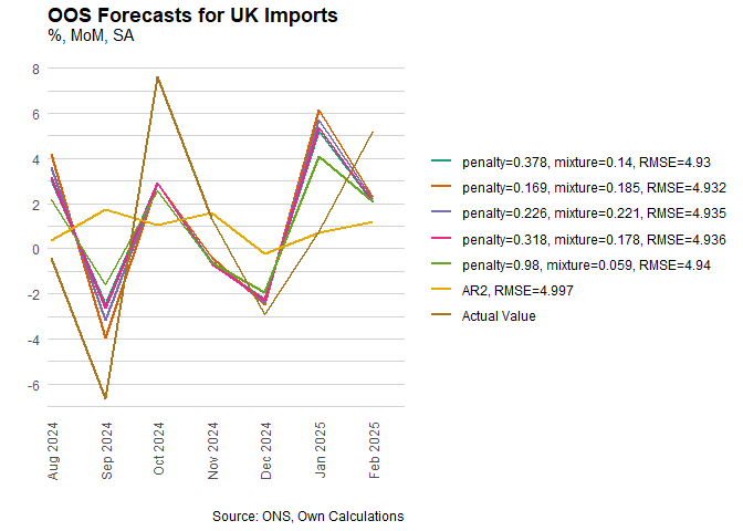
We compare the forecasts of the best Elastic Net configurations against the AR(2) benchmark.

The plot below shows predicted vs. actual import values across the out-of-sample forecast window. Notice that the RMSE for the top 5 models in lower when compared to the baseline AR.

db_graph <- results_glmnet %>% 
  mutate(name = paste0("penalty=",round(penalty,3),", mixture=",round(mixture,3),", RMSE=",round(mean,3),"")) %>% 
  arrange(mean) %>% 
  select(name, predictions) %>% 
  unnest(predictions) %>% 
  bind_rows(ar_predictions %>% mutate(name=paste("AR2, RMSE=",round(best_ar$mean,3), sep = ""))) %>% 
  mutate(name = factor(name, levels = .$name %>% unique)) 


g2 <-
  ggplot(db_graph, aes(x=date)) +
  geom_line(aes(y=.pred, color=name), linewidth=0.8) +
  geom_line(aes(y=Imports, color="Actual Value"), linewidth=0.8) +
  theme_minimal() + xlab("") + ylab("") +
  scale_color_brewer(palette = "Dark2") +
  scale_x_date(date_labels = "%b %Y",
               breaks = seq(from = as.Date(paste(year(min(db_graph$date)),
                                                 month(min(db_graph$date)),
                                                 "01",
                                                 sep="-")), 
                            to = max(db_graph$date),by = "month"),
               expand = expansion(mult = c(0.01,0.1))) +
  scale_y_continuous(n.breaks = 8) +
  labs(title="OOS Forecasts for UK Imports",
       subtitle = "%, MoM, SA",
       caption="Source: ONS, Own Calculations") +
  theme(panel.grid.major.x = element_blank(),
        panel.grid.minor.x = element_blank(),
        panel.grid.major.y = element_line(colour="lightgray", size=0.1),
        panel.grid.minor.y = element_line(colour="lightgray", size=0.1),
        axis.text.x = element_text(angle = 90, vjust = 0.5, hjust=1),
        plot.title=element_text(face="bold"),
        legend.title=element_blank()) +
  theme(
        plot.title = element_text(vjust = 1.5),
        plot.subtitle = element_text(vjust = 3.75)) +
  guides(col = guide_legend(direction = "vertical")) 

print(g2)

Adaptive Elastic Net

To refine variable selection and improve model sparsity, we estimate an Adaptive Elastic Net.

This method introduces feature-specific penalty weights, based on the coefficients from a an unpenalized estimation. This is usually the pure Ridge estimation, but as our best non-adaptative Elastic Net did not shrink any variable to zero, we can use it. These weights penalize less informative variables more heavily. The Adaptive Elastic Net should also have the oracle property in high dimensions, which the non-adaptative version lacks.

It is mathematically described in (Zou & Zhang, 2009) as:

\[\hat{\beta} = \arg\min_{\beta} \left\{ \frac{1}{2n} \| y - X\beta \|_2^2 + \lambda \left( \alpha \sum_{j=1}^p w_j |\beta_j| + \frac{1 - \alpha}{2} \|\beta\|_2^2 \right) \right\}\]

Where:

• \(w_j = \frac{1}{|\hat{\beta}^{(init)}_j|^\gamma}\) are adaptive weights
  from an initial estimator,
• \(\lambda\) and \(\alpha\) are the regularization strength and mixing
  parameter respectively,
• \(\gamma > 0\) controls the influence of the adaptive weights.

We repeat the tuning procedure with the new weights, seeking improved generalization and interpretability. Our weights are defined as the inverse of the coefficients estimated in the best non-adaptative model.

ada_factors <- results_glmnet$final_model[[1]]$fit %>% coefficients %>% .[-1] %>% as.numeric %>% abs() %>% {1/.}

tune_model_ada <- linear_reg(
  penalty = tune(), 
  mixture = tune()  
)


tune_model_ada <- do.call(set_engine,c(list(object = tune_model_ada, engine = "glmnet"), list(penalty.factor = ada_factors)))


wflow_ada <- workflow(preprocessor = formula, spec = tune_model_ada)

tune_results_ada <- tune_grid(wflow_ada, resamples = df_sampling, grid = grid,
               control = keep_pred, metrics = metric_set(rmse))

best_params_ada <- show_best(tune_results_ada, metric = "rmse")

We use the same do.call structures to organize all the relevant information in a nested tibble.

results_glmnet_ada <- best_params_ada %>%
  mutate(
    args = map2(penalty, mixture, ~list(penalty = .x, mixture = .y)),
    
    model_spec = map(args, ~ do.call(linear_reg, .x)),
    
    model_spec = map2(model_spec, penalty, ~ do.call(
      set_engine,
      c(list(object = .x, engine = "glmnet"), list(path_values = .y))
    )),
    
    final_wf = map(model_spec, ~ workflow(preprocessor = formula, spec = .x)),
    
    final_fit = map(final_wf, ~ last_fit(.x, split = df_full_sample)),
    
    final_model = map(final_fit, extract_fit_parsnip),
    
    predictions = map(final_fit, ~collect_predictions(.x) %>% 
   bind_cols(date = testing(df_full_sample)$date))
  )

db_graph <- results_glmnet_ada %>% 
  mutate(name = paste0("penalty=",round(penalty,3),", mixture=",round(mixture,3),", RMSE=",round(mean,3),"")) %>% 
  arrange(mean) %>% 
  select(name, predictions) %>% 
  unnest(predictions) %>% 
  bind_rows(ar_predictions %>% mutate(name=paste("AR2, RMSE=",round(best_ar$mean,3), sep = ""))) %>% 
  mutate(name = factor(name, levels = .$name %>% unique)) 


g3 <-
  ggplot(db_graph, aes(x=date)) +
  geom_line(aes(y=.pred, color=name), linewidth=0.8) +
  geom_line(aes(y=Imports, color="Actual Value"), linewidth=0.8) +
  theme_minimal() + xlab("") + ylab("") +
  scale_color_brewer(palette = "Dark2") +
  scale_x_date(date_labels = "%b %Y",
               breaks = seq(from = as.Date(paste(year(min(db_graph$date)),
                                                 month(min(db_graph$date)),
                                                 "01",
                                                 sep="-")), 
                            to = max(db_graph$date),by = "month"),
               expand = expansion(mult = c(0.01,0.1))) +
  scale_y_continuous(n.breaks = 8) +
  labs(title="OOS Forecasts for UK Imports",
       subtitle = "%, MoM, SA",
       caption="Source: ONS, Own Calculations") +
  theme(panel.grid.major.x = element_blank(),
        panel.grid.minor.x = element_blank(),
        panel.grid.major.y = element_line(colour="lightgray", size=0.1),
        panel.grid.minor.y = element_line(colour="lightgray", size=0.1),
        axis.text.x = element_text(angle = 90, vjust = 0.5, hjust=1),
        plot.title=element_text(face="bold"),
        legend.title=element_blank()) +
  theme(
        plot.title = element_text(vjust = 1.5),
        plot.subtitle = element_text(vjust = 3.75)) +
  guides(col = guide_legend(direction = "vertical")) 

print(g3)

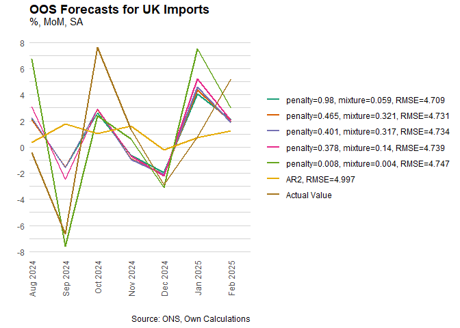
The new results have even lower RMSE than the non-adaptative models.

Regularization Path

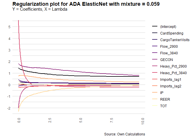
Finally, to understand the dynamic of model shrinkage, we trace the regularization path: the evolution of coefficient estimates as the penalty increases. For this exercise, we use the mixture parameter chosen by the best adaptative model.

This analysis highlights the relative importance and stability of each predictor as the model transitions from sparse to very regularized. It also reveals some puzzles regarding the coefficients. An increase in the real exchange rate, for example, has a negative effect on imports, which is difficult to justify based on economic theory. This is not a huge problem, as the goal of this exercise is not to perform inference, but to predict.

reg_path_grid <- grid_space_filling(
    penalty(range = c(-4,1)),
    type = "latin_hypercube",
    size = 200
)


reg_path <- reg_path_grid %>%
  mutate(
    args = map(penalty, ~list(penalty = .x, mixture = results_glmnet_ada$mixture[[1]])),
    
    model_spec = map(args, ~ do.call(linear_reg, .x)),
    
    model_spec = map2(model_spec, penalty, ~ do.call(
      set_engine,
      c(list(object = .x, engine = "glmnet"), list(path_values = .y, penalty_factors = ada_factors))
    )),
    
    final_wf = map(model_spec, ~ workflow(preprocessor = formula, spec = .x)),
    
    final_fit = map(final_wf, ~ last_fit(.x, split = df_full_sample)),
    
    final_model = map(final_fit, extract_fit_parsnip),
    
    coefficients = map(final_model, ~coefficients(.x$fit)),
    coefficients = map(coefficients, ~cbind(coefs = rownames(.x),
                                                            tibble(values = .x %>% as.matrix() %>%.[,1])))
  )
  
db_graph <- reg_path %>% 
  select(penalty, coefficients) %>% 
  unnest(coefficients)


g4 <-
  ggplot(db_graph, aes(x=penalty)) +
  geom_line(aes(y=values, color=coefs), linewidth=0.8) +
  theme_minimal() + xlab("") + ylab("") +
  scale_color_viridis_d(option = "magma") +
  scale_y_continuous(n.breaks = 8) +
  labs(title= paste0("Regularization plot for ADA ElasticNet with mixture = ",round(results_glmnet_ada$mixture[[1]],3),""),
       subtitle = "Y = Coefficients, X = Lambda",
       caption="Source: Own Calculations") +
  theme(panel.grid.major.x = element_blank(),
        panel.grid.minor.x = element_blank(),
        panel.grid.major.y = element_line(colour="lightgray", size=0.1),
        panel.grid.minor.y = element_line(colour="lightgray", size=0.1),
        axis.text.x = element_text(angle = 90, vjust = 0.5, hjust=1),
        plot.title=element_text(face="bold"),
        legend.title=element_blank()) +
  theme(
        plot.title = element_text(vjust = 1.5),
        plot.subtitle = element_text(vjust = 3.75)) +
  guides(col = guide_legend(direction = "vertical")) 

print(g4)

Conclusion

While the Elastic Net model does not achieve outstanding forecasting accuracy for the UK imports data, it consistently outperforms the baseline AR(2) model, even in a relatively data-constrained environment.

More importantly, this exercise demonstrates the construction of a robust pipeline for regularized time series modeling using tidymodels. The methodology includes cross-validation, adaptive penalization, and model comparison, offering a solid foundation for future forecasting tasks where variable selection and interpretability remain critical.